HQS Quantum Solver Documentation

Introduction to Electron Spectroscopy

The Jupyter notebooks corresponding to this section can be found here.

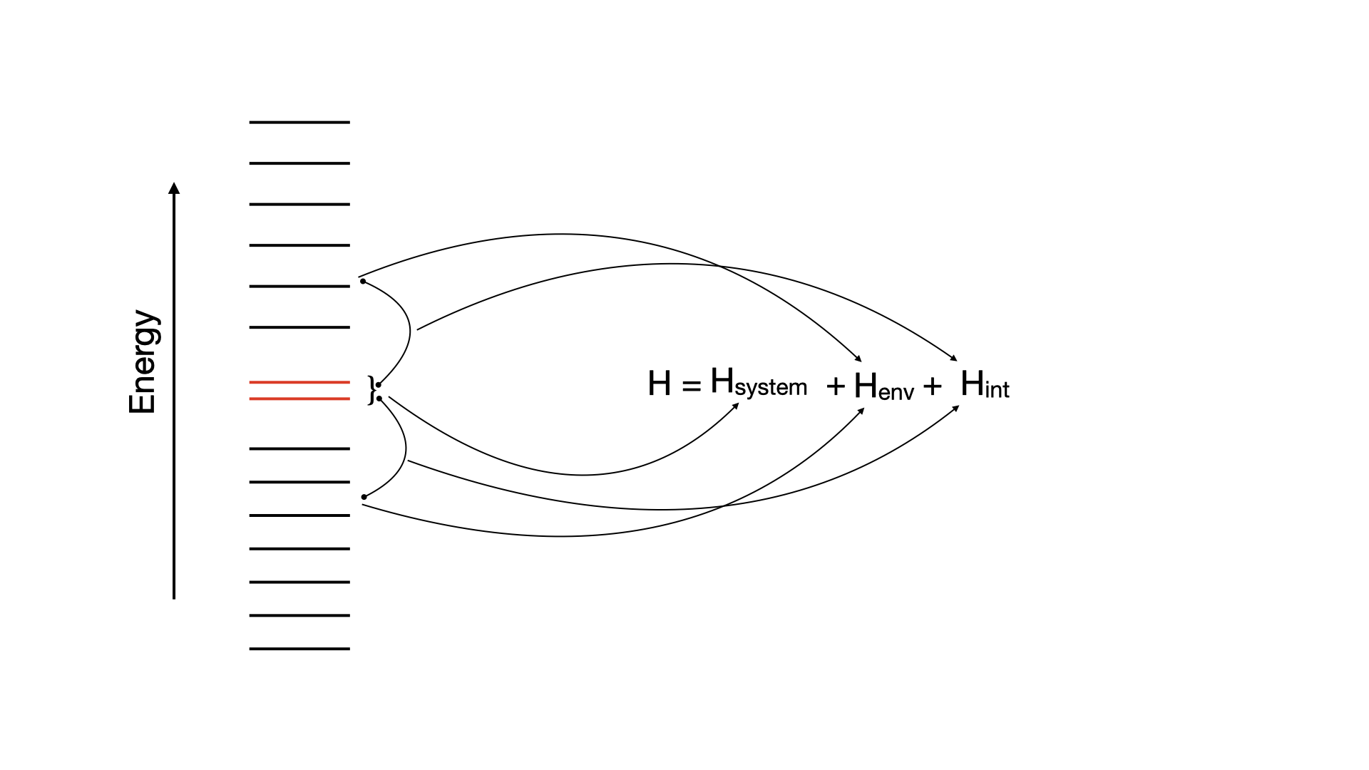
In this chapter, we calculate splittings, $\Delta E_{ST}$, of molecules using HQS Quantum Solver. The value $\Delta E_{ST}$ is the difference between the lowest singlet and the triplet electronic states of a molecule. The corresponding database contains specialized Hamiltonians for three molecules: furane, thiophene and cyclopentadiene, derived via random phase approximation (RPA). This method involves partitioning the system into an active space that interacts with the environment. The active subspace consists of two orbitals that interact with a bath made up of other molecular orbitals:

$$H=H_{12}+E_{env}+V.$$ NOTES:

• The Hamiltonian is derived in terms of qubits. The number of them can be varied and serves as an input parameter.
• One can return the full Hamiltonian or the truncated one, where number of qubits defines the truncation: the less qubits are available, the higher the truncation level.
• Hamiltonians are generated in the HQS Struqture format.
• The database also contains molecular structure and reference value of singlet-triplet splittings computed with quantum chemistry methods.

Imports & Parameters

To use HQS Quantum Solver and Struqture import the following:

from hqs_quantum_solver.spins import VectorSpace, Operator
from hqs_quantum_solver.spins import struqture_term
from electron_spectroscopy import Hamiltonians
from struqture_py.spins import PauliHamiltonian

Additionally import the following general-purpose libraries:

import numpy as np
import scipy.sparse as sparse
import matplotlib.pyplot as plt
from scipy.sparse.linalg import eigsh

Next, we need to import the electron_spectroscopy database and obtain one of the Hamiltonians:

from electron_spectroscopy import Hamiltonians

H = Hamiltonians.stored_hamiltonians["cyclopentadiene"]

Each Hamiltonian is a Python class containing numerical parameters.

Full Hamiltonians are currently computationally intractable, therefore, one should create a truncated one, restricted in number of qubits used for the environment. To create a truncated Hamiltonian in the struqture format run:

trunc_H = H.truncate_env(n_qubits=4, allow_large=False)

The maximum number of qubits to be solved by HQS Quantum Solver is 62. To generate more, one should set allow_large=True. The maximum number of qubits is equal to the length of the H.omega array and depends on the molecule. (In all examples this value is of the order of thousands.)

Alternatively, one may directly read-in a previously generated truncated Struqture Hamiltonian saved as a .json-file:

ham_json = "cyclopentadiene_4_qubits.json"
with open(ham_json, "r", encoding="utf-8") as f:
  trunk_H = PauliHamiltonian.from_json(f.read())

Reference Data

If you are interested in the molecular systems you are studying you can inspect the molecular geometries:

from electron_spectroscopy.xyzfiles import stored_structures

print(stored_structures["cyclopentadiene"])

To get a quantum chemistry reference value of singlet-triplet splitting and the information on the calculation run:

from electron_spectroscopy.data_dict import excitation_energies

print(excitation_energies["cyclopentadiene"])

Building Hamiltonian in HQS Quantum Solver

We first define the vector space for the system of two orbitals:

num_spins_cas = 2
v_cas = VectorSpace(sites=num_spins_cas, total_spin_z="all")

Then we create vector spaces for the bosonic bath for empty, single and double excitations in the bath:

v_bath_0 = VectorSpace(sites =num_spins_bath, total_spin_z=-num_spins_bath)
v_bath_1 = VectorSpace(sites=num_spins_bath, total_spin_z=-num_spins_bath + 2)
v_bath_2 = VectorSpace(sites=num_spins_bath, total_spin_z=-num_spins_bath + 4)
v_bath_3 = VectorSpace(sites=num_spins_bath, total_spin_z=-num_spins_bath + 6)
v_bath_4 = VectorSpace(sites=num_spins_bath, total_spin_z=-num_spins_bath + 8)

Now we build the complete vector space:

v_bath = v_bath_0   | v_bath_1 | v_bath_2 | v_bath_3 | v_bath_4
v = v_cas * v_bath

Finally, we convert the Struqture Hamiltonian directly to an HQS Quantum Solver operator

H = Operator(struqture_term(trunc_H), domain=v)

Solving the Hamiltonian

The Hamiltonian is solved by using the standard numerical machinery from the Python ecosystem:

k = min(10, H.shape[0] - 1)
eigenvalues, _ = eigsh(H, k=k, which="SA")

The singlet triplet gap $\Delta E_{ST}$ is a difference between first excited state energy (triplet) and ground state energy (singlet):

print("Singlet triplet gap:")
print ("E_t-E_g=", ( eigenvalues[1] - eigenvalues[0] ) * 27.2114,"eV")