Struqture Hamiltonians
The Jupyter notebook corresponding to this section can be found here.
In this guide you will learn how to create operators using Struqture, which is a library that is used to describe quantum mechanical operators and systems. It can be used as an input to HQS Quantum Solver for defining spin systems.
For this chapter, we use the system of antiferromagnetically coupled spins defined by the Hamiltonian , where
as an example.
Imports & Parameters
Throughout this chapter, we will use the following imports.
import numpy as np
import matplotlib.pyplot as plt
from scipy.sparse.linalg import eigsh

from struqture_py import PauliHamiltonian

from hqs_quantum_solver.spins import (
    VectorSpace, Operator, magnetic_field_z, struqture_term
)
Furthermore, we will make use of the following parameters.
M = 8    # number of sites/spins
J = 1.0  # interaction strength
B = 3.0  # magnetic field strength (will be introduced later)
Building Operators
Hamiltonians for spin systems can be described in Struqture using the PauliHamiltonian class. (Other options for describing spin systems are the PauliOperator and PlusMinusOperator classes.) The class describes a sum of products of operators. Each operator acts on a specific site of the system, and each product has at most one operator per site. More precisely, the operators have the form Inhere, , , and . The previously defined Hamiltonian can be written in this form: we have that which has the desired shape.
To define the Hamiltonian using Struqture, we first create an object of type
PauliHamiltonian and then add the individual products using the
.add_operator_product method.
Each product is given by a string, describing the operator product, and the
corresponding coefficient.
The string consecutively lists the terms of the product,
where each factor is represented by a number followed by a character.
The number defines the site the operator is acting on, and the character
defines the type of the operator, e.g. "2X3X" describes the product
.
In the following code, we use
Python format strings
to build the required strings.
interaction = PauliHamiltonian()

for j in range(M - 1):
    interaction.add_operator_product(f"{j}X{j+1}X", 0.25 * J)
    interaction.add_operator_product(f"{j}Y{j+1}Y", 0.25 * J)
    interaction.add_operator_product(f"{j}Z{j+1}Z", 0.25 * J)

print(interaction)
Running the code above creates the desired operator and prints the following output, which shows how Struqture stores the operator, where each line gives one summand from the formula for the Hamiltonian.
PauliHamiltonian{
0X1X: 5e-1,
0Y1Y: 5e-1,
0Z1Z: 5e-1,
1X2X: 5e-1,
1Y2Y: 5e-1,
1Z2Z: 5e-1,
2X3X: 5e-1,
2Y3Y: 5e-1,
2Z3Z: 5e-1,
3X4X: 5e-1,
3Y4Y: 5e-1,
3Z4Z: 5e-1,
4X5X: 5e-1,
4Y5Y: 5e-1,
4Z5Z: 5e-1,
5X6X: 5e-1,
5Y6Y: 5e-1,
5Z6Z: 5e-1,
}
Having a description of the Hamiltonian, we can create an actual operator
that we can use in computations. The first thing to do is to convert the
Struqture object into a Quantum Solver expression, using the
struqture_term function.
Then, we need to create a VectorSpace
object that described the vector space the operator is acting on, and
finally an
Operator
object, by passing in the expression describing the operator and the vector
space. Note that we can use the .current_number_spins method to set
the number of sites in the vector space.
v = VectorSpace(sites=interaction.current_number_spins(), total_spin_z="all")
hamiltonian = Operator(struqture_term(interaction), domain=v)
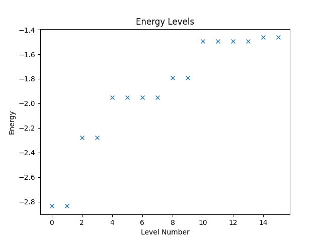
With the operator, we can now compute and plot the energy levels. Since Quantum Solver operators are compatible to SciPy, we can directly call the eigsh function from SciPy to obtain the energy levels. Then we use Matplotlib to create a plot of the levels.
eigvals, eigvecs = eigsh(hamiltonian, k=16, which="SA")

plt.figure("energy")
plt.title("Energy Levels")
plt.xlabel("Level Number")
plt.ylabel("Energy")
plt.plot(eigvals, "x")
The resulting figure is shown below.
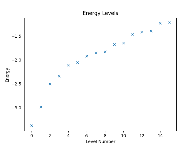
Restricting the Spin Polarization
If we know that we only need to consider states with a given total spin polarization in direction, e.g., when considering Hamiltonians that conserve the total spin polarization, we can restrict the states the vector space represents accordingly. This restriction can significantly reduce the amount of computational work needed. Say, we know that the total spin polarization is zero. Then, we can create the restricted vector space and the operator that is defined on it as follows.
w = VectorSpace(sites=interaction.current_number_spins(), total_spin_z=0)
hamiltonian2 = Operator(struqture_term(interaction), domain=w)
Computing and plotting the energy levels can then be done as before.
eigvals2, eigvecs2 = eigsh(hamiltonian2, k=16, which="SA")

plt.figure("energy-restricted")
plt.title("Energy Levels")
plt.xlabel("Level Number")
plt.ylabel("Energy")
plt.plot(eigvals2, "x")
Combining Expressions
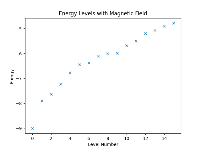
Next, we want to consider a slightly more complicated example. Assume that the spin system that we have defined at the beginning of this chapter is exposed to a magnetic field in direction of the -axis. More precisely, we want to consider the Hamiltonian that is given by
If we wanted, we could build the entire Hamiltonian using Struqture. There is, however, an easier way. Quantum Solver has already a definition of the magnetic-field term, namely the magnetic_field_z function. Furthermore, Quantum Solver allows building of arbitrary linear combination of Quantum Solver expressions. Hence, we can combine the Struqture definition of the spin interaction with the magnetic_field_z function, which is shown below.
hamiltonian3 = Operator(
    magnetic_field_z(coef=B * np.ones(v.sites)) + struqture_term(interaction),
    domain=w
)
Then, again, we can compute the energy levels and plot them.
eigvals3, eigvecs3 = eigsh(hamiltonian3, k=16, which="SA")

plt.figure("energy-with-field")
plt.title("Energy Levels with Magnetic Field")
plt.xlabel("Level Number")
plt.ylabel("Energy")
plt.plot(eigvals3, "x")

plt.show()
Finally, running the code produces the figure below.
Complete Code
# Title    : Using Struqture with HQS Quantum Solver
# Filename : struqture.py

# ===== Imports and Parameters =====

import numpy as np
import matplotlib.pyplot as plt
from scipy.sparse.linalg import eigsh

from struqture_py import PauliHamiltonian

from hqs_quantum_solver.spins import (
    VectorSpace, Operator, magnetic_field_z, struqture_term
)

M = 8    # number of sites/spins
J = 1.0  # interaction strength
B = 3.0  # magnetic field strength (will be introduced later)

# ===== Struqture Definition of the System =====

interaction = PauliHamiltonian()

for j in range(M - 1):
    interaction.add_operator_product(f"{j}X{j+1}X", 0.25 * J)
    interaction.add_operator_product(f"{j}Y{j+1}Y", 0.25 * J)
    interaction.add_operator_product(f"{j}Z{j+1}Z", 0.25 * J)

print(interaction)

# ===== Creating the Operator =====

v = VectorSpace(sites=interaction.current_number_spins(), total_spin_z="all")
hamiltonian = Operator(struqture_term(interaction), domain=v)

eigvals, eigvecs = eigsh(hamiltonian, k=16, which="SA")

plt.figure("energy")
plt.title("Energy Levels")
plt.xlabel("Level Number")
plt.ylabel("Energy")
plt.plot(eigvals, "x")

# ===== Restricted Sz =====

w = VectorSpace(sites=interaction.current_number_spins(), total_spin_z=0)
hamiltonian2 = Operator(struqture_term(interaction), domain=w)

eigvals2, eigvecs2 = eigsh(hamiltonian2, k=16, which="SA")

plt.figure("energy-restricted")
plt.title("Energy Levels")
plt.xlabel("Level Number")
plt.ylabel("Energy")
plt.plot(eigvals2, "x")

# ===== Combining Expressions =====

hamiltonian3 = Operator(
    magnetic_field_z(coef=B * np.ones(v.sites)) + struqture_term(interaction),
    domain=w
)

eigvals3, eigvecs3 = eigsh(hamiltonian3, k=16, which="SA")

plt.figure("energy-with-field")
plt.title("Energy Levels with Magnetic Field")
plt.xlabel("Level Number")
plt.ylabel("Energy")
plt.plot(eigvals3, "x")

plt.show()