Spin-Flip Simulation

In this guide, you will learn how to load the Hamiltonian of a spin system, compute the energy levels of the Hamiltonian, and simulate the evolution of the corresponding system in time. We will use the Hamiltonian describing Acrylonitride ( $C_{2} H_{3} CN$ ) in a magnetic field, as you would encounter, e.g., in an NMR spectrometer.

First, we need to import the functions, classes and modules that are required for the script. Therefore, we create a Python script and add the following imports to our file, which we will explain, as we go along.

# Title    : HQS Quantum Solver Spin Flip Simulation
# Filename : spin_flip.py
from pathlib import Path

import numpy as np
import matplotlib.pyplot as plt
from scipy.sparse.linalg import eigsh

from struqture_py.spins import PauliHamiltonian

from hqs_quantum_solver.spins import (
    VectorSpace, Operator, lowering, struqture_term, spin_z, raising
)
from hqs_quantum_solver.evolution import evolve_krylov, observers

Next, we load the Hamiltonian description from a file in Struqture format. Struqture is a library providing an exchage format for quantum operators. (See the "Struqture" section for more information about using Struqture with Quantum Solver.) We have to store the file acrylonitride.json (right click, "Save As..."), which contains the description of the Hamiltonian, in the same directory as the Python script. Afterwards, we can load it as follows.

filepath = Path("acrylonitride.json")
hamiltonian_info = PauliHamiltonian().from_json(filepath.read_text())

So far, we have only loaded a description of a Hamiltonian. To use it, we need to turn it into an actual Operator that, e.g., can be applied to a state vector. In addition to the definition of the operator, Quantum Solver needs the vector space that the operator is defined on to construct the operator. Since we are dealing with a spin system, we create a VectorSpace object from the spins module. Vector spaces, as used in quantum mechanics, are defined by the states they represent. The states of the system are defined by the site and the total_spin_z arguments. The former sets the number of spins in the system, and the latter can be used to only include states with a given total spin polarization. Since we want to include all states, we set total_spin_z to "all".

v = VectorSpace(sites=hamiltonian_info.current_number_spins(), total_spin_z="all")

Having constructed the vector space, we can now create an instance of type Operator.

hamiltonian = Operator(struqture_term(hamiltonian_info), domain=v, dtype=complex)

Herein, we used the struqture_term function to tell Quantum Solver that the input is in Struqture format. Furthermore, we enforced the construction of a complex-valued operator by setting dtype to complex. (Setting dtype is optional, but since we want to compute a time evolution of the system, which requires complex state vectors, having a complex operator yields better performance.)

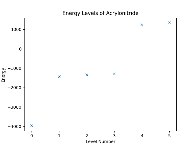
We can now obtain the energy levels of the system by computing the eigenvalues of the operator. The Operator class is compatible to SciPy, such that we can directly call the eigsh on the operator, and then use Matplotlib to plot the result.

eigvals, eigvecs = eigsh(hamiltonian, k=6, which="SA")

plt.figure("energy-levels")
plt.title("Energy Levels of Acrylonitride")
plt.xlabel("Level Number")
plt.ylabel("Energy")
plt.plot(eigvals, "x")

Running the script up to this point should result in an image as shown below.

We shall now turn to the simulation of the time evolution of the system described by the Hamiltonian. The first thing that we need is to setup the initial wave function of the system. For that, we want to take the groundstate of the system and flip one of the spins. Flipping the $j$ th spin is done by applying the operator $(\hat{S}_{j}^{+} + \hat{S}_{j}^{-})$ , which needs to be built first.

Quantum Solver has a selection of high-level functions that can be used to describe operators. For our purpose we use the raising and lowering functions, which describe the $\hat{S}^{+}$ and $\hat{S}^{-}$ operator, respectively. Since Quantum Solver allows for building of arbitrary linear combinations of those operator descriptions, we can build the desired spin-flip operator for the site with index 2 as follows.

flip = Operator(raising(site=2) + lowering(site=2), domain=v, dtype=complex)

The spin-flip operator can be applied to a wave function by using the .dot method of the operator.

groundstate = eigvecs[:, 0]
initial_wavefunction = flip.dot(groundstate)

Since inspecting the wave function directly is usually not very insightful, we need to perform an additional step, before we run a time simulation. We want to look at the expectation value of observables, in this case the spin polarizations $\hat{S}_{j}^{z}$ for all sites of the system. The operator $\hat{S}_{j}^{z}$ is described by the spin_z function, and we can create a list of all desired observables in the following way.

observables = [
    Operator(spin_z(site=j), domain=v, dtype=complex) for j in range(v.sites)
]

With the observables at hand, we can now create an array containing the time values at which we want to evaluate the wave function, call the evolve_krylov function to perform the simulation, and then stack the list of observations into a single NumPy array.

ts = np.linspace(0, 1e-1, 100)
result = evolve_krylov(
    hamiltonian, initial_wavefunction, ts,
    observer=observers.expectation(observables)
)
observations = np.stack(result.observations)

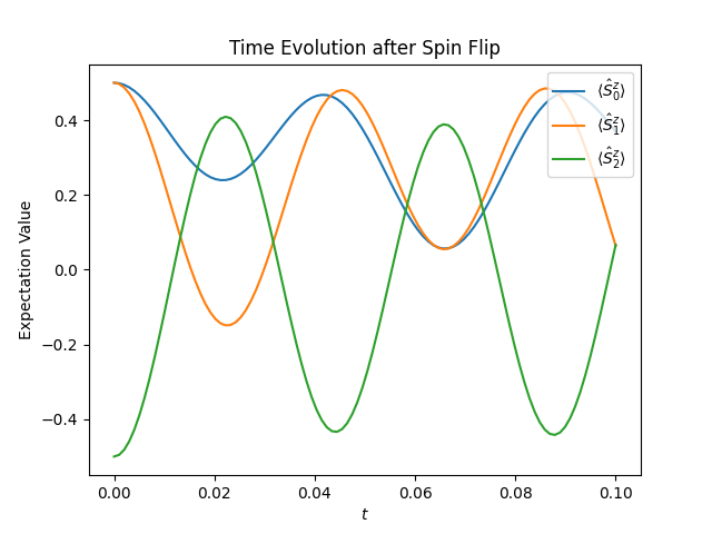
The result can then be visualized using the code below.

plt.figure("time-evolution")
plt.title("Time Evolution after Spin Flip")
plt.xlabel("$t$")
plt.ylabel("Expectation Value")
for j in range(observations.shape[1]):
    plt.plot(ts, observations[:, j], label=f"$\\langle \\hat{{S}}^z_{j} \\rangle$")
plt.legend(loc="upper right")
plt.show()

The figure below shows the resulting plot, which shows how the spins polarization oscillates after the spin flip.

Plot of the time evolution of the spin system.

Complete Code

# Title    : HQS Quantum Solver Spin Flip Simulation
# Filename : spin_flip.py
from pathlib import Path

import numpy as np
import matplotlib.pyplot as plt
from scipy.sparse.linalg import eigsh

from struqture_py.spins import PauliHamiltonian

from hqs_quantum_solver.spins import (
    VectorSpace, Operator, lowering, struqture_term, spin_z, raising
)
from hqs_quantum_solver.evolution import evolve_krylov, observers

# ===== Loading and Building the Hamiltonian =====

filepath = Path("acrylonitride.json")
hamiltonian_info = PauliHamiltonian().from_json(filepath.read_text())

v = VectorSpace(sites=hamiltonian_info.current_number_spins(), total_spin_z="all")
hamiltonian = Operator(struqture_term(hamiltonian_info), domain=v, dtype=complex)

# ===== Energy Levels =====

eigvals, eigvecs = eigsh(hamiltonian, k=6, which="SA")

plt.figure("energy-levels")
plt.title("Energy Levels of Acrylonitride")
plt.xlabel("Level Number")
plt.ylabel("Energy")
plt.plot(eigvals, "x")

# ===== Spin Flip =====

flip = Operator(raising(site=2) + lowering(site=2), domain=v, dtype=complex)

groundstate = eigvecs[:, 0]
initial_wavefunction = flip.dot(groundstate)

# ===== Time Evolution =====

observables = [
    Operator(spin_z(site=j), domain=v, dtype=complex) for j in range(v.sites)
]

ts = np.linspace(0, 1e-1, 100)
result = evolve_krylov(
    hamiltonian, initial_wavefunction, ts,
    observer=observers.expectation(observables)
)
observations = np.stack(result.observations)

plt.figure("time-evolution")
plt.title("Time Evolution after Spin Flip")
plt.xlabel("$t$")
plt.ylabel("Expectation Value")
for j in range(observations.shape[1]):
    plt.plot(ts, observations[:, j], label=f"$\\langle \\hat{{S}}^z_{j} \\rangle$")
plt.legend(loc="upper right")
plt.show()

Keyboard shortcuts

HQS Quantum Solver Documentation

Spin-Flip Simulation

Complete Code