Introduction

HQS Spectrum Tools is a software toolkit to simulate NMR spectra. It consists of hqs-nmr, containing simulation tools and hqs-nmr-parameters, providing NMR parameters for a variety of molecules. With HQS Spectrum Tools you can calculate and analyze NMR spectra for molecules or other spin systems. Given the NMR parameters of a molecule, a simple python API can be used to calculate the associated NMR spectrum. RUST and C++ components are used internally to achieve remarkable speed and accuracy, even for complex, large molecules.

HQS Spectrum Tools is also an integral part of HQSpectrum, our end-to-end solution for NMR spectra analysis, which is available to you, if you have an existing HQStage account.

NMR spectra prediction is also a very promising use case for the quantum computer. To explore this possibility, we offer to extract the relevant spin Hamiltonians in struqture format for all molecules in the hqs-nmr-parameters database.

If you are interested in the theory behind NMR or the math of how to calculate NMR spectra, take a look at the background chapter.

Applications

Nuclear magnetic resonance (NMR) spectroscopy is a key analytical tool in chemistry and related disciplines. Its broad application not only facilitates the identification of molecules, but also provides intricate details about their structure, dynamics, and chemical environment. The ability to compare an experimental NMR spectrum with theoretical predictions for various compounds is crucial for the accurate identification and characterization of chemical entities.

Our NMR spectrum solvers are designed for both speed and precision. They are based on a very efficient implementation in the frequency domain. With a variety of solver strategies at your disposal, you can leverage symmetries and clustering techniques either fully automated or customized according to your specifications. This flexibility allows you to tailor your approach based on the specific characteristics of your system, optimizing performance without sacrificing accuracy.

Getting started

To use HQS Spectrum Tools you need a running version of HQStage. You can check here how to set it up. Once you have HQStage correctly configured you can install HQS Spectrum Tools using the command:

hqstage install hqs-nmr

Please note that HQS Spectrum Tools is currently only supported on Linux.

For some of the functionalities of HQS Spectrum Tools (especially the provided example NMR parameters), the RDKit cheminformatics package is required. While packages are available on pypi.org, at present they are not officially supported by the RDKit development team. Therefore, it is strongly recommended to install it via the conda-forge channel to ensure the access to its latest version. The easiest way to install the library is running the following command in an active conda environment:

conda install rdkit

The following code snippet can be used to create your first program using HQS Spectrum Tools. For an expanded collection of examples please see the examples section.

from hqs_nmr.calculate import calculate_spectrum
from hqs_nmr.datatypes import NMRCalculationParameters
from hqs_nmr.visualization import plot_spectrum
from hqs_nmr_parameters.examples import molecules

from matplotlib import pyplot as plt


# Obtain example molecule of datatype NMRParameters.
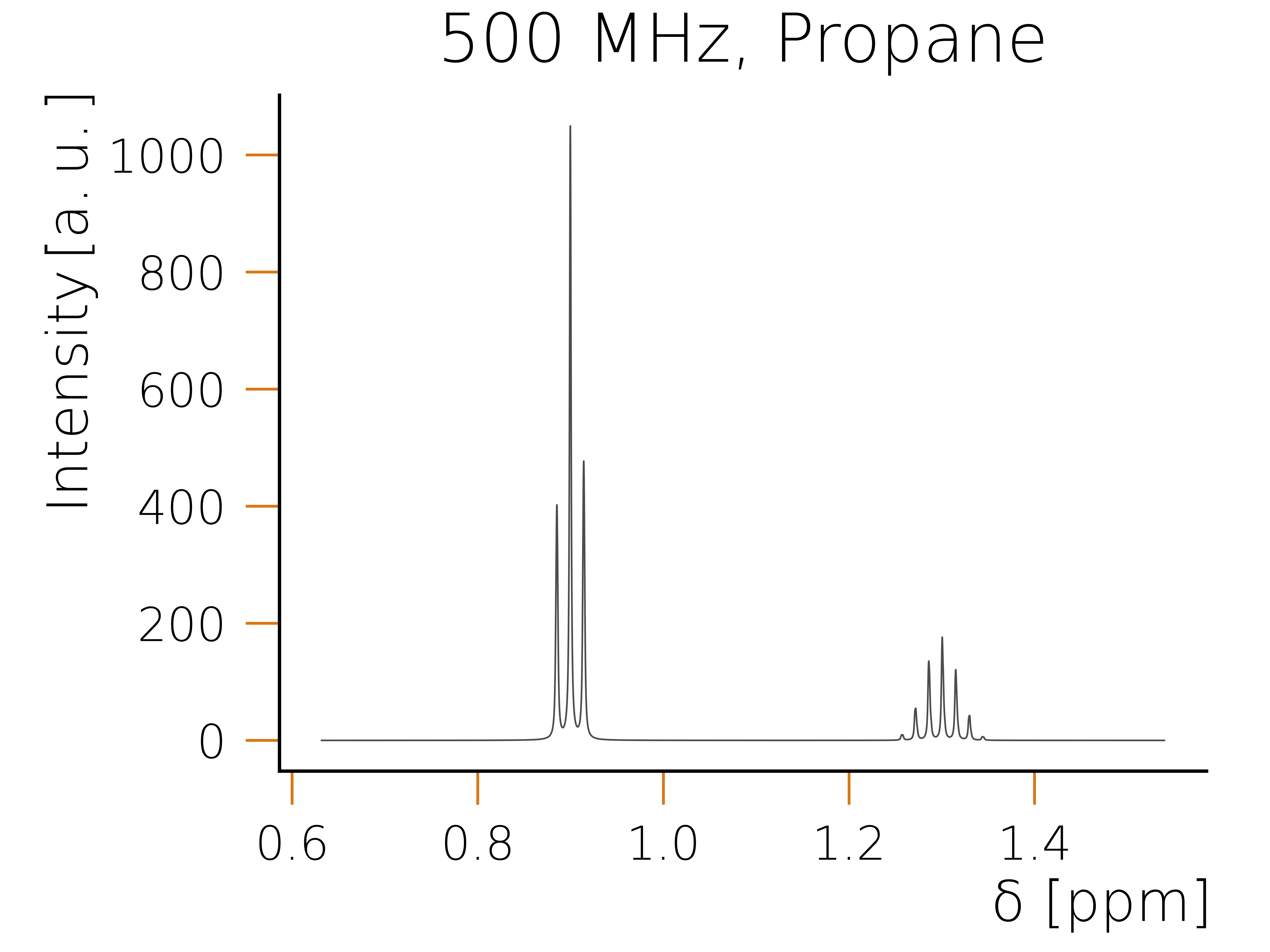
molecule_parameters = molecules["C3H8"].spin_system()

# Define the calculation parameters. The only required field is the magnetic
# field in Tesla
calculation_parameters = NMRCalculationParameters(field_T=11.7433)

# Calculate the individual spin contributions of the spectrum.
nmr_result = calculate_spectrum(
    molecule_parameters,
    calculation_parameters
)

# Plot the spectrum.
plot_spectrum(nmr_result.spectrum)
plt.show()

Executing the code snippet using python should result in the following plot:

Features

• Frequency domain-based fast and precise NMR spectra calculation.
• Automatic implementation to compute accurate 1D NMR spectra with minimal truncation errors for large numbers of spins, featuring linear scaling with system size.
• NMR example parameters (chemical shifts and J-couplings) for molecules of different sizes, accessible via data classes containing structural information.
• Custom NMR parameters can be specified conveniently for NMR spectrum simulation.
• Easy construction of an NMR Spin Hamiltonian from provided or custom parameters using the struqture-py package.
• Extensive customization options of the NMR solver for expert users.
• Postprocessing methods to analyze simulated spectra and compare them to experiment.

You can get an overview of the HQS Spectrum Tools Python library in the components chapter or take a look at the API-documentation.

Getting started

The best way to learn about HQS Spectrum Tools is to go through our example notebooks. You can find information on how to download and run the examples in the local usage section of our HQStage documentation. Alternatively you can take a look at the executed notebooks in the hqstage-examples public github repository.

The following notebooks provide brief introductions to the software if you are new to it.

• 1_getting_started: Introduces the main routines of HQS Spectrum Tools. These are mostly automated and include all you need to simulate NMR spectra.

• 2_hqs_nmr_parameters_introduction: Introduces the hqs-nmr-parameters database and shows how to retrieve the spin Hamiltonian in struqture format for the available molecules.

Further examples

For a more detailed introduction into HQS Spectrum tools, the following advanced example notebooks are available:

• 3_customization: Explains customization options, e.g., to decrease runtime or improve resolution by discussing the solver strategies employed. This includes the clustering approach and the frequency-based implementation.

• 4_hqs_nmr_parameters_in_detail: A detailed overview of the functionalities of hqs-nmr-parameters as well as the available datasets.

• 5_plot_spectra_hqsnmr_exp: Demonstrates how to compare the calculated spectra to experimental results.

• 6_high_symmetry_molecules: Details the special case of a highly symmetric, strongly coupled molecule where the clustering approach fails and how to obtain the correct result.

Using struqture and the solver backend

In case you want to try out your own approximation schemes or customize the solver backend, check out the following examples:

• 7_spectrum_from_struqture_hamiltonian: Elaborates on how to interface with the solver backend given an NMR spin Hamiltonian in struqture format and how to use the spin-dependent clustering approach.

• 8_spin_lattice_models: Showcases how to extend the provided functionality to spin lattice models.

• 9_user_defined_solver: Allows to add a custom solver to the framework provided by HQS Spectrum Tools.

• 10_nmr_using_struqture_and_qiskit: Example on how to calculate an NMR spectrum on a quantum computer using struqture and qiskit.

Background

This chapter provides an overview of the fundamentals behind HQS Spectrum Tools

In section NMR, we describe the basics of nuclear magnetic resonance (NMR) from an experimental and theoretical perspective. We discuss, for example, the different relevant parameters entering an NMR calculation, such as the chemical shifts or couplings between nuclear spins, and introduce the relevant Hamiltonian of a molecule for NMR.

In Mathematical Background, we describe in greater detail the math behind calculation of spectra in HQS Spectrum Tools.

Finally, in the section Calculating NMR Spectra, we discuss approaches for evaluating NMR spectra of large molecules.

NMR

Nuclear magnetic resonance (NMR) spectroscopy is one of the most important analytical techniques in chemistry and related fields. It is widely used to identify molecules, but also to obtain information about their structure, dynamics, and chemical environment.

For a detailed overview to the field there are many suitable textbooks like High Resolution NMR Techniques in Organic Chemistry by T. Claridge or Understanding NMR Spectroscopy by J. Keeler. However, in the following we will only summarize some fundamental aspects of NMR which should be sufficient to get you started to use HQS Spectrum Tools.

NMR spectrometers place the sample into a strong, but constant magnetic field and use a weak electromagnetic pulse to perturb the nuclei. At or near resonance, when the oscillation frequency matches the intrinsic frequency of a nucleus, the system responds by producing an electromagnetic signal with a frequency characteristic of the magnetic field at the respective nucleus.

The NMR Hamiltonian used to simulate NMR spectra as well as the effects leading to the intrinsic frequency of a nucleus are discussed below, while the origin of the electromagnetic signal as well as a possible experimental setup are discussed in detail in section Measurement of a 1D NMR spectrum.

Zeeman interaction

For the simulation of NMR spectra for molecules, the most important part is the Zeeman effect describing the interaction of the nuclear spin with the external magnetic field $\mathbf{B}$. The corresponding Hamiltonian can be written as

$$\begin{array}{r}{\hat{H}}_{\text{Z}}=-\gamma \mathbf{B}\cdot \hat{\mathbf{S}},\end{array}$$

where $\gamma$ is the gyromagnetic ratio, the ratio of a system's magnetic moment to its angular momentum, and $\hat{\mathbf{S}}=({\hat{S}}^x,{\hat{S}}^y,{\hat{S}}^z{)}^{\text{T}}$ is the total spin operator. Assuming that the strong (and constant) magnetic field is in $z$-direction only, meaning $\mathbf{B}=(0,0,B^z)$, the Hamiltonian simplifies to

$$\begin{array}{r}{\hat{H}}_{\text{Z}}=-\gamma B^z{\hat{S}}^z={\omega }_0{\hat{S}}^z,\end{array}$$

where ${\omega }_0=-\gamma B^z$ is the so-called Larmor frequency, the angular frequency corresponding to the precession of the spin magnetization around the magnetic field at the position of the nucleus.

As an example, consider the simplest nucleus, ¹H, consisting of only one proton, for which the gyromagnetic ratio is $\gamma /2\pi =42.6$ MHz T⁻¹, meaning that a 500 MHz NMR spectrometer has a static magnetic field of about 11.7 Tesla. The energy of radiation of the Larmor frequency $\nu =500$ MHz ($h\nu \approx 3.3\cdot 10^{-25}$ J) is several orders of magnitude smaller than the average thermal energy of a molecule at a temperature of $T=298$ K ($k_{\text{B}}T\approx 4.1\cdot 10^{-21}$ J). Therefore, the occupations of the spin states are almost equal at room temperature, only a small surplus is responsible for the sample magnetization.

Chemical shift

Perhaps the most important aspect for NMR spectroscopy in chemistry is that the nuclei in molecules are shielded against the external magnetic field by the electrons surrounding them. This can be expressed by adding a correction term to the Hamiltonian as

$$\begin{array}{r}{\hat{H}}_{\text{Z}}=-\gamma (1-\mathbf{\sigma })\mathbf{B}\cdot \hat{\mathbf{S}},\end{array}$$

where $\mathbf{\sigma }$ is referred to as the shielding tensor quantifying the change in the local magnetic field experienced by the nucleus in the molecule relative to a bare nucleus in vacuum. A significant simplification occurs if the molecules of interest are in solution, or in liquid phase in general, as they can rotate freely and only the isotropic shielding $\sigma =\frac{1}{3}\text{Tr}(\mathbf{\sigma })$ is of interest,

$$\begin{array}{r}{\hat{H}}_{\text{Z}}=-\gamma (1-\sigma )B^z{\hat{S}}^z.\end{array}$$

In practice, chemical shifts are normally used instead of chemical shieldings: instead of invoking the Larmor frequency of a nucleus in vacuum, shifts are defined with respect to the resonance frequency ${\nu }_{\text{ref}}$ of a reference compound:

$$\begin{array}{r}\delta =\frac{\nu -{\nu }_{\text{ref}}}{{\nu }_{\text{ref}}}\approx {\sigma }_{\text{ref}}-\sigma ,\end{array}$$

The standard reference for ¹H NMR is the Larmor frequency of the protons in TMS [tetramethylsilane, Si(CH₃)₄]. Chemical shifts are normally reported on a scale of ppm (parts per million): most ¹H chemical shifts are observed in the range between 0 and 10 ppm, and most ¹³C chemical shifts between 0 and 200 ppm. Since a constant shift of the form $\gamma {\sigma }_{\text{ref}}{B}^z\hat{S}$ leaves the spectrum unchanged up to a scaling factor and the scale of chemical shieldings is so small in absolute terms $\left(|\sigma |\ll 1\right)$, for practical intents and purposes the chemical shift can be substituted directly into the Hamiltonian:

$$\begin{array}{r}{\hat{H}}_{\text{Z}}=-\gamma (1+\delta )B^z{\hat{S}}^z.\end{array}$$

Spin-spin coupling

Up to this point, the nuclear spins have been regarded to be isolated from each other. However, their magnetic moments have an effect on neighboring spins. The interaction of the nuclear spins can happen through two different mechanisms. The first one is the direct (or through space) spin-spin coupling, where the interaction strength depends on the distance of the two nuclei and the angle of their distance vector relative to the external field. As it comes from the direct interaction of two magnetic dipoles, it is also referred to as dipolar coupling. However, the effect is generally not observable in liquid phase since the free rotation of the molecules averages over all orientations and thus results in a vanishing average coupling.

An effect observable in the NMR spectrum is indirect spin-spin coupling, which is mediated by the electrons of a chemical bond. Due to the Pauli principle, the electrons of a covalent bond always have an anti-parallel spin orientation, and one electron will be closer to one nucleus than to the other, preferring an anti-parallel orientation with the nearby nucleus. Depending on the number of electrons involved in the transmission of the interaction, either a parallel or an anti-parallel orientation of two nuclei may result in a lower energy. Importantly, this interaction does not average out in solution since it mainly depends on the electron density at the position of the nucleus and not on the orientation of the distance vector relative to the field, which is why it is also referred to as scalar coupling. Since only s-orbitals have a finite electron density at the nucleus, the coupling depends on the electron density in those orbitals alone.

The interaction Hamiltonian in the case of homonuclear coupling is given by

$$\begin{array}{r}{\hat{H}}_J=2\pi \hslash J{\hat{\mathbf{I}}}_1\cdot {\hat{\mathbf{I}}}_2,\end{array}$$

where $\hat{\mathbf{I}}={\hslash }^{-1}\hat{\mathbf{S}}$.

It should be noted that the $\mathbf{J}$-coupling tensor is a real $3\times 3$ matrix that depends on the molecular orientation, but in liquid phase only its isotropic part $J$ is observed due to motional averaging. Typical $J$-coupling strengths between protons in ¹H NMR amount to a few Hz.

NMR spin Hamiltonian for molecules in liquid phase

The spin Hamiltonian in a static magnetic field in frequency units (rad s⁻¹) is given by

$$\begin{array}{r}\hat{H}={\hslash }^{-1}({\hat{H}}_{\text{Z}}+{\hat{H}}_J)=-\sum _k{\gamma }_k(1+{\delta }_k)B^z{\hat{I}}_k^z+2\pi \sum _{k<l}{J}_{kl}{\hat{\mathbf{I}}}_k\cdot {\hat{\mathbf{I}}}_l,\end{array}$$

where the sum runs over all nuclear spins of interest.

There are several interactions that have not been taken into account here. As already mentioned, the direct dipolar spin-spin interaction vanishes in liquids due to motional averaging. Beyond dipolar coupling, such as quadrupolar interactions, for instance, are relevant only for nuclei with spin quantum number $I\ge 1$. Furthermore, interactions with unpaired electrons need a special treatment as well. While most organic compounds are diamagnetic (closed-shell), paramagnetic NMR also exists.

Mathematical Background

The Hamiltonian $\hat{H}$ we are using for the NMR systems is of the form

$$\begin{array}{r}\hat{H}=-\sum _l{\gamma }_l\left(1+{\delta }_l\right)B^z{\hat{I}}_l^z+2\pi \sum _{k<l}{J}_{kl}{\hat{\mathbf{I}}}_k\cdot {\hat{\mathbf{I}}}_l,\end{array}$$

where ${\gamma }_{\ell }$ are the gyromagnetic factors and ${\delta }_{\ell }$ the chemical shifts of nuclear spin $\ell$. $J_{kl}$ denotes the coupling between spins $k$ and $l$ and ${\hat{I}}^{\alpha }={\hat{S}}^{\alpha }/\hslash$ where the ${\hat{S}}^{\alpha }$ are the usual $\mathrm{SU}(2)$ spin operators with $\alpha \in \{x,y,z\}$.

Note in the following, whenever we denote a spin operator as ${\hat{I}}^{\alpha }$ without an additional site index, we mean the sum over the individual spin operators for each nuclear spin ${\hat{I}}^{\alpha }={\sum }_i{\hat{I}}_i^{\alpha }$.

In NMR spectroscopy, there is a strong magnetic field $B^z$ in the $z$-direction, and electromagnetic pulses / oscillating fields are applied to flip the spins into the $x/y$-plane. $B^z$ is typically of the order of 500 MHz, the bandwidth of the pulses is about 10 kHz, and the required resolution is less than 1 Hz.

The spectrum measured in an NMR experiment corresponds to the spectral function calculated in HQS Spectrum Tools.

Measurement of a 1D NMR spectrum

A 1D NMR spectrum can be obtained using a pulse-acquire experiment. To discuss how to calculate it, we will first elaborate on how the experiment is performed. For this, after a probe has been placed inside an NMR spectrometer, a strong magnetic field is applied along the $z$-axis, which leads to a net magnetization along the same axis. Note that at room temperature this magnetization is typically quite small. One then applies a $\pi /2$-pulse along the $x$-axis which flips the magnetization to the minus $y$-direction. The spins then start to precess in the $xy$-plane, which creates a signal that can be recorded by measuring the magnetic field along the $x$- or $y$-axis. The induced magnetic field ${\mathbf{B}}^{xy}$ is directly linked to the magnetization $\mathbf{M}$ of the sample as

$$\begin{array}{r}{\mathbf{B}}^{xy}(t)={\mu }_0{\mathbf{M}}^{xy}(t),\end{array}$$

which in turn can be linked to the magnetic moment $\mathbf{m}$

$$\begin{array}{r}{\mathbf{m}}^{xy}(t)=\int {\mathbf{M}}^{xy}(t)\mathrm{d}V={\mathbf{M}}^{xy}(t)V,\end{array}$$

where the integral goes over the volume $V$ of the sample and we are assuming a uniform magnetization within the sample to evaluate the integral. At the same time, the magnetic moment of an individual molecule is given as

$$\begin{array}{r}{\mathbf{m}}^{xy}(t)=⟨\sum _k{\gamma }_k{\hat{\mathbf{S}}}_k^{xy}⟩(t).\end{array}$$

Therefore, to calculate the spectrum, we simply have to calculate the time-dependent expectation value of the nuclear spin operators of each spin along the $x$- or $y$-direction and scale them with the corresponding gyromagnetic ratio. Note that in the actual implementation we perform the calculation using the dimensionless nuclear spin operator, so we explicitly calculate

$$\begin{array}{r}⟨\sum _k{\gamma }_k{\hat{I}}_k^{xy}⟩(t)={\hslash }^{-1}⟨\sum _k{\gamma }_k{\hat{\mathbf{S}}}_k^{xy}⟩(t).\end{array}$$

The sum of these contributions is directly proportional to the measured magnetic field. To obtain the absolute measured magnetic field, an additional scaling would be required based on information on the sample volume and concentration of the molecule. However, this scaling is typically unnecessary as one is not interested in absolute values. So in HQS Spectrum Tools the spectrum is by default normalized to integrate to the number of relevant spins, i.e., to those of the same isotope type as the reference isotope.

Calculation of the spectrum

Time domain

Let us now discuss how to evaluate these expectation values. For this, we will only consider the field along the $x$-direction. The time-dependent expectation value can be calculated using the density operator $\hat{\rho }(t)$

$$\begin{array}{r}⟨{\gamma }_k{\hat{I}}_k^x⟩(t)=\mathrm{Tr}\left({\gamma }_k{\hat{I}}_k^x\hat{\rho }(t)\right).\end{array}$$

Where $\mathrm{Tr}(...)$ denotes the trace. This implies that we need to find an expression for the time evolution of the density operator, which is described by the Liouville-von-Neumann equation

$$\begin{array}{r}\frac{\mathrm{d}\hat{\rho }}{\mathrm{d}t}=\frac{i}{\hslash }[\hat{H},\hat{\rho }].\end{array}$$

In this formulation the equation assumes a Hamiltonian in units of Joule, however the Hamiltonian as defined above is in units of radians per second, which allows us to drop the $\hslash$ factor. Therefore the time evolution can be written as

$$\begin{array}{r}\hat{\rho }(t)=e^{-i\hat{H}t}\hat{\rho }(t_0)e^{i\hat{H}t},\end{array}$$

which can easily be verified by reinserting this expression into the Liouville-von-Neumann equation. Note that $\hat{H}$ is the Hamiltonian of the process taking place within the time interval $[t_0,t]$. Therefore we have to perform two time evolutions: we start with the density operator at some time $t_0$ and perform a time evolution using the Hamiltonian associated with the $\pi /2$ pulse. Then we perform a second time evolution using the NMR Hamiltonian, describing the precession of the spins in the $xy$-plane.

Due to the setup of the experiment we can assume a hard (or instantaneous) pulse, meaning we will not be interested in the explicit time evolution during the pulse and can therefore write the time evolution operator of the pulse as

$$\begin{array}{r}{\hat{P}}_{\pi /2}^x=e^{-i\frac{\pi }{2}{\hat{I}}^x}.\end{array}$$

This leads to the following density operator after the pulse

$$\begin{array}{r}\hat{\rho }(t_p)={\hat{P}}_{\pi /2}^x\hat{\rho }(t_0)({\hat{P}}_{\pi /2}^x{)}^{†},\end{array}$$

where $t_p$ is the time duration of the pulse. Performing the second time evolution under the NMR Hamiltonian we arrive at

$$\begin{array}{r}\hat{\rho }(t)=e^{-i\hat{H}t}\hat{\rho }(t_p)e^{i\hat{H}t}=e^{-i\hat{H}t}{\hat{P}}_{\pi /2}^x\hat{\rho }(t_0)({\hat{P}}_{\pi /2}^x{)}^{†}{e}^{i\hat{H}t}.\end{array}$$

We now just have to define the density operator at time $t_0$. Due to the experimental setup it is simply given via the Boltzmann distribution

$$\begin{array}{r}\hat{\rho }(t_0)=\frac{e^{-\beta \hslash \hat{H}}}{Z}\end{array}$$

with the inverse temperature $\beta =\frac{1}{k_{\text{B}}T}$, where $k_{\text{B}}$ is the Boltzmann constant and $T$ the temperature, as well as the partition function $Z$. Note that the factor $\hslash$ is necessary as the Hamiltonian $\hat{H}$ is given in units of radians per second.

While HQS Spectrum Tools provides a solver that evaluates a spectrum using the exact expression of the density operator, one should note that for typical NMR experiments it is sufficient to approximate it using a series expansion of the exponential

$$\begin{array}{r}\hat{\rho }(t_0)=\frac{e^{-\beta \hslash \hat{H}}}{Z}\approx \frac{1}{Z}(I-\beta \hslash \hat{H})\approx \frac{1}{Z}-\frac{\beta \hslash B^z}{Z}\sum _l{\gamma }_l(1+{\delta }_l){\hat{I}}_l^z.\end{array}$$

In the second approximation applied here, the second term is replaced by the magnetic field term of the Hamiltonian. This is valid as the contribution from the J-coupling term to the distribution is insignificant in comparison. Furthermore, the first term with the identity $I$ can be dropped in practical calculations as it does not contribute to the overall expectation value.

Note that in the NMR literature this step is often skipped and sometimes even ${\hat{I}}^z$ is called a density operator. This is technically incorrect as ${\hat{I}}^z$ is not positive semi-definite, a key requirement for a density operator. Furthermore, the prefactor $\frac{\beta \hslash B^z}{Z}$ is often omitted, as it only serves as normalization.

However, with this approximation one can now further simplify the calculation using the identity

$$\begin{array}{r}{\hat{P}}_{\alpha }^x{\hat{I}}^z({\hat{P}}_{\alpha }^x{)}^{†}=e^{-i\alpha {\hat{I}}^x}{\hat{I}}^z{e}^{i\alpha {\hat{I}}^x}=\cos (\alpha ){\hat{I}}^z+i\sin (\alpha )[{\hat{I}}^z,{\hat{I}}^x],\end{array}$$

which in our case of a $\pi /2$-pulse reduces to

$$\begin{array}{r}{\hat{P}}_{\pi /2}^x{\hat{I}}^z({\hat{P}}_{\pi /2}^x{)}^{†}=-{\hat{I}}^y.\end{array}$$

This leads us to the final expression for the expectation value

$$\begin{array}{rl}⟨{\gamma }_k{\hat{I}}_k^x⟩(t)& =\mathrm{Tr}\left({\gamma }_k{\hat{I}}_k^x\hat{\rho }(t)\right)\\ & =\mathrm{Tr}\left({\gamma }_k{\hat{I}}_k^x{e}^{-i\hat{H}t}{\hat{P}}_{\pi /2}^x\hat{\rho }(t_0)({\hat{P}}_{\pi /2}^x{)}^{†}{e}^{i\hat{H}t}\right)\\ & \approx \frac{1}{Z}\mathrm{Tr}\left({\gamma }_k{\hat{I}}_k^x{e}^{-i\hat{H}t}{\hat{P}}_{\pi /2}^x(1-\beta \hslash B^z\sum _l{\gamma }_l(1+{\delta }_l){\hat{I}}_l^z)({\hat{P}}_{\pi /2}^x{)}^{†}{e}^{i\hat{H}t}\right)\\ & =\frac{\beta \hslash B^z}{Z}{\gamma }_k\sum _l{\gamma }_l(1+{\delta }_l)\mathrm{Tr}\left({\hat{I}}_k^x{e}^{-i\hat{H}t}{\hat{I}}_l^y{e}^{i\hat{H}t}\right).\end{array}$$

Where, as mentioned above, in the last step we dropped the term arising from the identity in the parentheses, since it does not contribute to the overall expectation value.

Frequency domain

Up to now we have only discussed how to calculate the time signal, however what we are actually interested in is the spectrum given by its Fourier transform. Most implementations therefore first calculate a time evolution according to the derivation performed above and then do a Fourier transform of the result. However, as will be explained in the next section, it is much more efficient to do the Fourier transform analytically first and then perform all calculations in the frequency domain. To be able to do this, we have to rewrite the above formulation into a so called Lehmann representation

$$\begin{array}{rl}⟨{\gamma }_k{\hat{I}}_k^x⟩(t)& =\frac{\beta \hslash B^z}{Z}{\gamma }_k\sum _l{\gamma }_l(1+{\delta }_l)\mathrm{Tr}\left({\hat{I}}_k^x{e}^{-i\hat{H}t}{\hat{I}}_l^y{e}^{i\hat{H}t}\right)\\ & =\frac{\beta \hslash B^z}{Z}{\gamma }_k\sum _l{\gamma }_l(1+{\delta }_l)\sum _n⟨n|{\hat{I}}_k^x\sum _m|m⟩⟨m|e^{-i\hat{H}t}{\hat{I}}_l^y{e}^{i\hat{H}t}|n⟩\\ & =\frac{\beta \hslash B^z}{Z}{\gamma }_k\sum _l{\gamma }_l(1+{\delta }_l)\sum _{n,m}⟨n|{\hat{I}}_k^x|m⟩⟨m|{\hat{I}}_l^y|n⟩e^{i(E_n-E_m)t},\end{array}$$

where $|m⟩$ and $|n⟩$ are the eigenvectors of the NMR Hamiltonian constructed in a many-body spin basis with the respective eigenvalues $E_m$ and $E_n$. These can be obtained from numerical diagonalization using standard dense linear algebra routines. By introducing a small convergence aiding factor $\eta$ we can now do the Fourier transform

$$\begin{array}{rl}⟨{\gamma }_k{\hat{I}}_k^x⟩(\omega )& =\int e^{i(\omega +i\eta )t}⟨{\gamma }_k{\hat{I}}_k^x⟩(t)\mathrm{d}t\\ & =\frac{\beta \hslash B^z}{Z}{\gamma }_k\sum _l{\gamma }_l(1+{\delta }_l)\sum _{n,m}⟨n|{\hat{I}}_k^x|m⟩⟨m|{\hat{I}}_l^y|n⟩\int e^{i(\omega +i\eta +E_n-E_m)t}\mathrm{d}t\\ & =\frac{\beta \hslash B^z}{Z}{\gamma }_k\sum _l{\gamma }_l(1+{\delta }_l)\sum _{n,m}\frac{⟨n|{\hat{I}}_k^x|m⟩⟨m|{\hat{I}}_l^y|n⟩}{i(\omega +i\eta +E_n-E_m)}\\ & =-i\frac{\beta \hslash B^z}{Z}{\gamma }_k\sum _l{\gamma }_l(1+{\delta }_l)\sum _{n,m}\frac{⟨n|{\hat{I}}_k^x|m⟩⟨m|{\hat{I}}_l^y|n⟩}{\omega +i\eta +E_n-E_m}.\end{array}$$

This represents the final form we are evaluating, although for the spectrum we are measuring in NMR, typically just the real part is required. However for some postprocessing routines also the imaginary part is required, in which case we will refer to this as a Green's function.

Additionally, note that the factor $\eta$ leads to a broadening of the peaks, giving them generally the shape of a Lorentzian. This broadening has to be chosen to fit the expected resolution, as discussed in the next section.

Energy rediscretization

One problem that arises when simulating NMR spectra is that the peaks are usually very sharp, which means that resolving them numerically poses a challenge in itself. Therefore, performing calculations in time domain typically requires a lot of time steps that have to be evaluated. Also in the frequency domain, discretizing the frequency axis with a very fine grid would be computationally ineffective. Therefore, we perform several rounds of computing the spectral function and use the result of each round to rediscretize the frequency grid for the next. We first calculate the spectral function with a linear grid in frequency space and a rather large artificial broadening $\eta$. Based on this result we rediscretize the frequency space in equal weight partitions of the total spectral function. This gives us a new non-linear frequency grid with grid points accumulated around the spectral function peaks. We then repeat this process with a smaller broadening $\eta$, which allows us to resolve sharper peaks. This way, we can iteratively reach the desired resolution.

Calculating NMR Spectra

While using the Lehmann representation for the expectation value

$$\begin{array}{rl}⟨{\gamma }_k{\hat{I}}_k^x⟩(\omega )& =-i\frac{\beta \hslash B^z}{Z}{\gamma }_k\sum _l{\gamma }_l(1+{\delta }_l)\sum _{n,m}\frac{⟨n|{\hat{I}}_k^x|m⟩⟨m|{\hat{I}}_l^y|n⟩}{\omega +i\eta +E_n-E_m}\end{array}$$

is useful to resolve sharp features in an NMR spectrum, it does not address the problem of the exponential scaling of the Hamiltonian dimension. Evaluating this expression in a brute force approach would imply diagonalizing a Hamiltonian of dimension $2^M$ where $M$ is the number of spins in the molecule. This would restrict one to around 10 spins on a modern laptop. Therefore, different strategies need to be employed to evaluate NMR spectra for larger molecules.

Symmetry

First one can use the fact that the NMR Hamiltonian always conserves the $I^z$ quantum number, which means that we can identify a block diagonal structure in the Hamiltonian, where each block can be diagonalized individually. While this is always possible for the standard NMR Hamiltonian, it only restricts the dimension of the largest block to $\left(\genfrac{}{}{0ex}{}{M}{M/2}\right)$ which still grows rather quickly.

For some molecules one can also identify magnetically equivalent groups. Such a symmetry group is defined as a group of spins, where each individual spin has the same chemical shift and couples in the exact same way to the rest of the system. Identifying these groups is advantageous, as one can combine them into higher order spin representations, which allows to exploit the local $\mathrm{SU}(2)$ symmetry of these groups. As an example consider a propane molecule, which has eight hydrogen atoms. By identifying all symmetrically coupled groups in this molecule, the number of spins can be reduced to two. One being the CH₂ group which has a combined spin representation of one and the second being the two methyl groups each representing a spin 3/2 and adding up to a total spin representation of spin 3. As the corresponding operators ${\hat{I}}^2$ of these two combined spins commute with the Hamiltonian, we can construct a basis in which the Hamiltonian has again a block diagonal structure, however the individual blocks are even smaller, as when exploiting just the $I^z$ conservation.

While these symmetry considerations are exact and can lead to a reasonable reduction in computational effort, they eventually break down when going to larger and larger molecules. Therefore, also approximate methods have to be used.

Clustering methods

The main approximation method used in HQS Spectrum Tools is based on the observation that we do not just evaluate the full sum over spin contributions to the spectrum at once, but rather determine the contribution of each individual spin separately. This allows us to identify an effective Hamiltonian for each spin and evaluate the spectral function for it independently from the other spin contributions. It turns out that a good approximation for the Hamiltonian for a specific spin contribution is typically given by simply identifying the cluster of spins most strongly coupled to the spin of interest. A good measure for this coupling is the following weight matrix, motivated from perturbation theory

$$\begin{array}{r}{\Delta }_{kl}=\frac{J_{kl}^2}{({\gamma }_k{\delta }_k-{\gamma }_l{\delta }_l)B^z}\end{array}$$

Here, $J_{kl}$ are the entries in the J-coupling matrix connecting spins with index $k$ and $l$, ${\gamma }_{k/l}$ the gyromagnetic ratios, ${\delta }_{k/l}$ the chemical shift values, and $B^z$ the magnetic field strength in $z$-direction.

Especially at high field, this method is extremely accurate allowing to choose cluster sizes around 8–12 spins for basically all molecules.

Database

In this section we will give an overview of the hqs-nmr-parameters database. In molecular data, we will introduce the molecular data structure, which is used as input in HQS Spectrum Tools and involves:

• Chemical name and molecular formula
• Chemical structures
• Conditions of the experiment/simulation
• NMR parameters

Next, it is shown how to extract the relevant spin Hamiltonian from this input.

Then, the various datasets available within hqs-nmr-parameters are discussed.

Finally, we will demonstrate how to provide external data as text input to use the functionalities of HQS Spectrum Tools for your own molecules, where we are using custom Pydantic data classes to ensure consistency.

Representation in Python of molecular data structures

Molecular data

Inside the hqs-nmr-parameters package, the MolecularData class, which is derived from Pydantic's BaseModel, has been implemented to describe a molecule. It contains the following attributes:

• name: The name of the molecule (just a simple string).
• isotopes: List containing pairs of an atom index and the associated isotope. Atom indices are associated with the order in which atoms appear in the chemical structure representations, starting by index 0.
• shifts: List containing pairs of an atom index and the associated chemical shift in ppm.
• j_couplings: List containing pairs of atomic indices and the associated J-coupling values in Hz. Note that atom index pairs are unique: if a value is provided for an atom pair (k, l), then no value is provided for pair (l, k).
• structures: Contains a dictionary with chemical structure representations. It accepts entries for a SMILES string ("SMILES"), a Molfile ("Molfile"), and an XYZ file ("XYZ"). Each value will correspond to a ChemicalStructure object. See below for a full explanation of the chemical structure representations and the atom numeration.
• formula: The molecular formula of the corresponding molecule.
• temperature: An optional temperature in K for which the parameters have been calculated or at which the experiment has been performed.
• solvent: Name of the solvent. An empty string represents an unknown or undefined solvent, or the absence of a solvent.
• description: Optional further information.
• method_json: Stores a JSON serialization of computational method settings. An empty string indicates that the field is not applicable. Creating and interpreting the content is the responsibility of the user of the model.

This is best illustrated by an example from one of our available datasets:

# Import a MolecularDataSet
from hqs_nmr_parameters.examples import molecules

# Choose ethanol as an example from the available molecules
parameters = molecules["C2H5OH"]

print(type(parameters))
print("Chemical name:", parameters.name)
print("Molecular Formula:", parameters.formula)
print("Type(s) of representations:", parameters.structures.keys())
print("Information about solvent:", parameters.solvent)
print("Shifts:", parameters.shifts)
print("###")
print(parameters.description)

<class 'hqs_nmr_parameters.code.data_classes.MolecularData'>
Chemical name: Ethanol
Molecular Formula: C2H6O
Type(s) of representations: dict_keys(['SMILES'])
Information about solvent: chloroform
Shifts: [(3, 1.25), (4, 1.25), (5, 1.25), (6, 3.72), (7, 3.72), (8, 1.32)]
###
1H parameters for ethanol in CDCl3.
Shifts from: https://doi.org/10.1021/om100106e
J-couplings estimated.

In this case, we are getting information for the ethanol molecule, for which we have stored a SMILES representation (check below for details) and according to the description experimental ¹H NMR parameters in chloroform.

Note that the number of H atoms in a molecule is not necessarily the same as the number of spins in its ¹H NMR spectrum simulation. For instance, H atoms attached to electronegative elements such as N, O, or S tend to exchange rapidly with the deuterium atoms in protic solvents such as deuterated water (D₂O), which results in an extreme line broadening in the NMR spectrum or even makes the signal disappear entirely. That means, if the ethanol entry shown above was recorded in water instead of chloroform, the chemical shift value for the hydroxyl proton (OH, index 8) would probably be missing.

NMR parameters subset

The easiest way to check the NMR data is getting only the information necessary to perform an NMR calculation, i.e., a subset of the parameters object containing only the attributes isotopes, shifts, and j_couplings. Those can be obtained using the spin_system method of MolecularData, which returns an object of type NMRParameters:

from pprint import pprint
from hqs_nmr_parameters.examples import molecules

parameters = molecules["C2H5OH"]
nmr_parameters = parameters.spin_system()

print(type(nmr_parameters))
pprint(nmr_parameters.model_dump())

<class 'hqs_nmr_parameters.code.data_classes.NMRParameters'>
{'isotopes': [(1, 'H'), (1, 'H'), (1, 'H'), (1, 'H'), (1, 'H'), (1, 'H')],
 'j_couplings': [((0, 3), 7.0),
                 ((0, 4), 7.0),
                 ((1, 3), 7.0),
                 ((1, 4), 7.0),
                 ((2, 3), 7.0),
                 ((2, 4), 7.0)],
 'shifts': [1.25, 1.25, 1.25, 3.72, 3.72, 1.32]}

Here, nmr_parameters is an instance of the Pydantic NMRParameters class, where the atomic indices always start from 0. The total number of spins, determined from the number of chemical shifts, can be accessed with the nspins property. The NMRParameters class can be used as input for several functions to calculate an NMR spectrum, which is explained here in detail. The following code block shows how to perform a ¹H NMR simulation (default case), providing the molecular data either as NMRParameters or directly as MolecularData object:

from hqs_nmr_parameters.examples import molecules
from hqs_nmr import calculate_spectrum, NMRCalculationParameters

parameters = molecules["C2H5OH"]
nmr_parameters = parameters.spin_system()
print(type(nmr_parameters))
print(nmr_parameters.nspins)
calculation_parameters = NMRCalculationParameters(field_T=9.395)

# Using parameters instead of nmr_parameters would also be valid
spectrum = calculate_spectrum(nmr_parameters, calculation_parameters)
print(type(spectrum))

<class 'hqs_nmr_parameters.code.data_classes.NMRParameters'>
6
<class 'hqs_nmr.datatypes.NMRResultSpectrum1D'>

For information on the output class NMRResultSpectrum1D have a look here.

Isotopes/atoms selection

MolecularData objects can contain data for several isotopes. However, we are often interested in creating a spin system for a given nucleus only. For example, if we want to simulate a ¹H NMR spectrum but we also have ¹³C NMR parameters in our data, it is possible either to select only ¹H using keep_nuclei(isotopes=["1H"]) or to drop ¹³C using drop_nuclei(isotopes=["13C"]). Let us take a look at this in more detail:

from pprint import pprint
from hqs_nmr_parameters.examples import molecules

parameters = molecules["CH3Cl_13C"]
pprint(parameters.isotopes)

drop_C = parameters.drop_nuclei(isotopes=["13C"])
keep_H = parameters.keep_nuclei(isotopes=["1H"])
print(drop_C == keep_H)

nmr_parameters_1H = drop_C.spin_system()
pprint(nmr_parameters_1H.model_dump())

[(0, Isotope(mass_number=13, symbol='C')),
 (2, Isotope(mass_number=1, symbol='H')),
 (3, Isotope(mass_number=1, symbol='H')),
 (4, Isotope(mass_number=1, symbol='H'))]
True
{'isotopes': [(1, 'H'), (1, 'H'), (1, 'H')],
 'j_couplings': [((0, 1), -10.8), ((0, 2), -10.8), ((1, 2), -10.8)],
 'shifts': [3.05, 3.05, 3.05]}

We should take into account that the dropping/keeping of isotopes needs to be done carefully. The ¹³C nucleus has a nuclear spin of 1/2 (like ¹H) and is NMR-activate but has a very low natural abundance, and the ¹³C–¹H coupling pattern is only barely visible in ¹H NMR spectra. Therefore, it is common to simulate only ¹³ C-decoupled ¹H NMR spectra. However, the coupling of ¹H with other isotopes such as ¹⁹F or ³¹P should not be ignored in order to get the correct peak pattern.

keep_nuclei can also take an atoms argument, which accepts a list of atom indices for which the NMR parameters are to be kept. In the case of drop_nuclei, specified nuclei can be dropped via atoms, but a keep_atoms argument prevents certain atoms from being dropped (useful in combination with isotopes).

Note that many datasets provided by hqs-nmr-parameters already only contain the data that is needed to simulate ¹H NMR spectra. More information on each dataset can be found here.

Molecular structure representations

As shown above a MolecularData object has the attribute structures, which is a dictionary that can accept three entries (keys): "SMILES", "Molfile" and "XYZ". The value of each of these entries is a ChemicalStructure object that stores chemical structure representations of the type defined in the key:

• SMILES (Simplified Molecular-Input Line-Entry System): Strings representing the connectivity of all non-hydrogen atoms in a molecule. They become laborious to understand for complex molecules.
• Molfiles: Text files with a two-dimensional (2D) structure of a molecule (skeletal representation). It may omit hydrogen atoms. The number of hydrogen atoms is inferred from the atomic valencies of the heavy atoms.
• XYZ files: Text files containing an integer with the total number of atoms in the first line, followed by a comment line, and then the chemical element symbols and three-dimensional atomic positions for all the atoms explicitly.

Connectivity and charge information can be extracted from SMILES strings or Molfiles, but not from XYZ files. More information about Molfiles and SMILES can be found here.

The attributes of the ChemicalStructure class are:

• representation: Type of chemical structure representation present in the content attribute. It can be "SMILES", "Molfile" or "XYZ".
• content: The raw structure representation (as a string), i.e., a SMILES string or the content of an XYZ file or a Molfile.
• charge: Total net electric charge of the molecule.
• symbols: List of chemical element symbols for the full set of atoms.
• atom_map: As we have seen, 2D representations can omit hydrogen atoms, this attribute contains information about how the full representation would map into this reduced representation. It is a list of the length of the molecule (full set of atoms), where the atom counting starts from zero and takes into account:
  • Each non-hydrogen atom maps onto the respective index in the reduced representation.
  • Each explicit hydrogen maps onto the index of its explicitly represented counterpart.
  • Each implicit hydrogen maps onto the reduced index of the respective backbone atom.

In the case of ethanol, a full structures representation may look like the following. It might look a bit crowded as the content attribute contains the full content of the corresponding files (or SMILES string):

from hqs_nmr_parameters import ChemicalStructure

ethanol_representation = {
"XYZ": ChemicalStructure(representation="XYZ", content="9\n\nC       -0.88708900     0.17506400    -0.01253500\nC        0.46048900    -0.51551600    -0.04653500\nO        1.44296500     0.30726700     0.56557200\nH       -0.84747800     1.12776800    -0.55081700\nH       -1.65878200    -0.45332700    -0.46584200\nH       -1.17694400     0.40367600     1.01830600\nH        0.76871200    -0.72432800    -1.07546000\nH        0.41948600    -1.46207300     0.50017700\nH        1.47864000     1.14146800     0.06713500\n", charge=0, symbols=["C", "C", "O", "H", "H", "H", "H", "H", "H"], atom_map=[0, 1, 2, 3, 4, 5, 6, 7, 8]),
"Molfile": ChemicalStructure(representation="Molfile", content="\n     RDKit          2D\n\n  0  0  0  0  0  0  0  0  0  0999 V3000\nM  V30 BEGIN CTAB\nM  V30 COUNTS 3 2 0 0 0\nM  V30 BEGIN ATOM\nM  V30 1 C -1.299038 -0.250000 0.000000 0\nM  V30 2 C 0.000000 0.500000 0.000000 0\nM  V30 3 O 1.299038 -0.250000 0.000000 0\nM  V30 END ATOM\nM  V30 BEGIN BOND\nM  V30 1 1 1 2 CFG=3\nM  V30 2 1 2 3 CFG=3\nM  V30 END BOND\nM  V30 END CTAB\nM  END\n", charge=0, symbols=["C", "C", "O", "H", "H", "H", "H", "H", "H"], atom_map=[0, 1, 2, 0, 0, 0, 1, 1, 2]),
"SMILES": ChemicalStructure(representation="SMILES", content="CCO", charge=0, symbols=["C", "C", "O", "H", "H", "H", "H", "H", "H"], atom_map=[0, 1, 2, 0, 0, 0, 1, 1, 2])
}

Each of the entries corresponds to a ChemicalStructure object:

from pprint import pprint

smiles_representation = ethanol_representation["SMILES"]
print(type(smiles_representation))
pprint(smiles_representation.model_dump())

<class 'hqs_nmr_parameters.code.data_classes.ChemicalStructure'>
{'atom_map': [0, 1, 2, 0, 0, 0, 1, 1, 2],
 'charge': 0,
 'content': 'CCO',
 'representation': 'SMILES',
 'symbols': ['C', 'C', 'O', 'H', 'H', 'H', 'H', 'H', 'H']}

ethanol_representation["Molfile"].atom_map and ethanol_representation["SMILES"].atom_map will return:

[0, 1, 2, 0, 0, 0, 1, 1, 2]

In both cases, only the carbon and the oxygen atoms have been indicated explicitly. Therefore, the first three atoms are listed expressly (carbon atoms 0 and 1, and oxygen atom 2, i.e., the atom counting starts from zero) and the six following hydrogens are assigned to one of those backbone atoms. The full atomic indices associated with each reduced index can be obtained using the inverted_map method:

from pprint import pprint

smiles_representation = ethanol_representation["SMILES"]
print(smiles_representation.atom_map)
print(smiles_representation.inverted_map)

[0, 1, 2, 0, 0, 0, 1, 1, 2]
[{0, 3, 4, 5}, {1, 6, 7}, {8, 2}]

Hence, C (index = 0) is connected to H atoms 3, 4, 5, while C (index = 1) is connected to H atoms 6, 7, and the O (index = 2), to H 8.

However, ethanol_representation["XYZ"].atom_map will return:

[0, 1, 2, 3, 4, 5, 6, 7, 8]

Since all the atoms are explicitly provided in an XYZ format.

The ChemicalStructure class can also yield the chemical formula in Hill notation using the formula method. smiles_representation.formula will return:

'C2H6O'

Serialization (saving in a JSON file) of a MolecularData object and deserialization

We can save a MolecularData instance in a JSON file for future uses. To do so, employ the write_file method of the MolecularData class:

from hqs_nmr_parameters.examples import molecules

parameters = molecules["C2H5OH"]
parameters.write_file("etoh_molecular_data.json")

This JSON file can easily be loaded and validated against the MolecularData model using the read_file method:

from hqs_nmr_parameters import MolecularData

loaded_parameters = MolecularData.read_file("etoh_molecular_data.json")
print(type(loaded_parameters))

<class 'hqs_nmr_parameters.code.data_classes.MolecularData'>

Spin Hamiltonian

With the molecular data or just the NMR parameters mentioned in the previous section, it is possible to set up the spin Hamiltonian of the spin system relevant for an NMR simulation. This can be achieved by calling the hqs_nmr_parameters.nmr_hamiltonian function that returns the spin Hamiltonian defined in a struqture format. It contains the terms normally needed to represent the spin Hamiltonian of a closed-shell organic molecule in solution:

• Zeeman interaction of nuclei with the static magnetic field
• isotropic chemical shifts
• indirect spin-spin scalar couplings

Note that the units of the spin Hamiltonian conform to the conventions in the field of NMR. In consequence, the Hamiltonian is in angular frequency units of rad s⁻¹. To convert to Hz, the Hamiltonian needs to be divided by 2π. To convert to energy units (Joule), the Hamiltonian needs to be multiplied with the reduced Planck constant ℏ.

The parameters argument in nmr_hamiltonian can accept either a MolecularData or an NMRParameters object. For example, an NMR spin Hamiltonian with the example parameters for nitrobenzene at a field of 2.5 T can be set up as shown below (for information on how to retrieve the molecular data from a dataset, see the next section):

from hqs_nmr_parameters import examples, nmr_hamiltonian

parameters = examples.molecules["C6H5NO2"]
hamiltonian = nmr_hamiltonian(parameters=parameters, field=2.5)

Furthermore, the following optional arguments can be set:

• reference_isotope: Used to set up a relative spin Hamiltonian for use within the rotating frame approximation. The Larmor frequency of the reference isotope is subtracted from the Zeeman terms of all nuclei. The default value is None, i.e., the full Hamiltonian will be set up instead.
• reference_shift: Shift in ppm for the reference frequency in the rotating frame approximation. It can help to evaluate the Hamiltonian in the correct range of frequencies. Default: 0.0.
• gyromagnetic_ratios: Gyromagnetic ratios in rad s⁻¹ T⁻¹ of relevant isotopes. Default: pre-saved values.

As mentioned above, the reference_isotope option should be set to construct the spin Hamiltonian in the rotating frame approximation. For example, using the Larmor frequency of ¹H with a shift of 0 ppm as the reference frequency (default), a spin Hamiltonian is obtained via:

from hqs_nmr_parameters import examples, nmr_hamiltonian

parameters = examples.molecules["C6H5NO2"]
hamiltonian_rf = nmr_hamiltonian(
    parameters=parameters,
    field=2.5,
    reference_isotope=(1, "H"),
)

As discussed in the Molecular data section, it is possible to drop terms related to, e.g., ¹³C isotopes. Here this is not necessary, as the examples.molecules dataset used here only contains ¹H NMR parameters for the selected molecule C6H5NO2.

For a more detailed introduction on how to set up and work with a spin Hamiltonian, please have a look at the example notebooks.

Datasets

This chapter gives an introduction to all datasets provided by hqs-nmr-parameters and the data structure that is used to retrieve them.

Data types

MolecularDataSet

Molecular data for a group of molecules can be collected using the MolecularDataSet Pydantic class, which contains instances of type MolecularData. It is composed of two attributes:

• description: Summary of the content of the dataset.
• dataset: Dictionary where the keys are identifiers for the molecules (e.g., molecule names) and the values correspond to a MolecularData object per molecule.

A list with the keys of the dataset can be obtained directly from the MolecularDataSet.keys property. This allows us to conveniently access the molecular data of each molecule using its key as string.

In oder to have a brief summary of the molecules belonging to a dataset, we can use the get_names method. It retrieves a dictionary where the keys correspond to the keys of the dataset and the values are the chemical names. An equivalent dictionary providing the chemical formulas can be accessed via the get_formulas method.

Similar to keep_nuclei/drop_nuclei in MolecularData, keep_isotopes, drop_isotopes keeps/drops selected isotopes for all molecules in a dataset. An extra description can be added with updated information about the set (whitespace for separation from the original description content must be included).

As in MolecularData, it is possible to save or load datasets thanks to the read_file and write_file methods that (de)serialize JSON files.

MolecularDataTable

It is possible to store multiple molecular datasets in one MolecularDataTable object. This is particularly useful if the datasets contain the same or partially the same molecular structures, but different NMR parameters, e.g., from theoretical calculations using different DFT approaches. A MolecularDataTable object has two attributes:

• description: Summary of the content of the data table.
• content: A dictionary with keys being row labels (e.g., molecular identifiers as in a MolecularDataSet) and the values being objects of type MolecularDataTableRow that store different NMR parameters for a single molecular structure.

The most important properties of this class are row_labels and column_labels providing the respective labels, where the rows correspond to molecular structures and the columns to a specific data source. With the get_column and get_dataset methods, a dictionary or a MolecularDataSet can be obtained from a table column by specifying its label. Other functions that are known from the MolecularDataSet also exist for the MolecularDataTable. These are, for instance, get_names, get_formulas, read_file, and write_file.

General remarks

The hqs-nmr-parameters package contains several datasets organized in modules with data from different origins and for different purposes. In general, the MolecularDataSet object of a specific set can be imported with:

from hqs_nmr_parameters.<module> import <dataset>

With the exception of assignments, all modules have a dataset called molecules, which is an alias for the dataset that is presumably the most interesting one for the majority of users and is therefore recommended for general use.

To import the different modules in a single MolecularDataSet object, one can do:

from hqs_nmr_parameters import molecules

which is equivalent to:

from hqs_nmr_parameters.merged import molecules

Including the one imported above, there are four datasets that integrate the data available in hqs-nmr-parameters in some way:

• molecules: Includes all available molecules with any data, using experimental shifts if possible.
• calculated: Includes all available molecules that contain purely calculated parameters (shifts and J-couplings).
• combined: Includes all available molecules for which a combination of experimental shifts and calculated J-couplings is available.
• free_trial: Includes data available in the free trial version of HQSpectrum (calculated data from CHESHIRE and examples).

The datasets used here are described in more detail below along with the most important methods to access their contents. These methods (and properties) are accessible for each dataset, including the merged ones presented here.

Examples module

The first dataset that is worth mentioning is the examples module which has a set of molecule definitions encapsulated in the MolecularDataSet object molecules. This set can be accessed via:

from pprint import pprint
from hqs_nmr_parameters.examples import molecules

print(type(molecules)) # MolecularDataSet
# Keys of the dataset:
print(molecules.keys)

<class 'hqs_nmr_parameters.code.data_classes.MolecularDataSet'>
['CH3Cl', 'limonene_DFT', '1,2,4-trichlorobenzene', 'Anethole', 'Artemisinin_exp', 'endo-dicyclopentadiene_DFT', 'CH3Cl_13C', 'C2H3CN', 'Artemisinin', 'camphor_DFT', 'C6H6', 'C10H8', 'Triphenylphosphine_oxide', 'H2CCF2', 'C2H5Cl', 'Androstenedione', 'Cinnamaldehyde', 'CHCl3_13C', 'C6H5NO2', 'C2H5OH', 'C2H6', 'C10H7Br', 'CHCl3', 'camphor_exp', 'exo-dicyclopentadiene_DFT', '1,2-di-tert-butyl-diphosphane', 'C2H3NC', 'cyclopentadiene_DFT', 'cis-3-chloroacrylic_acid_exp', 'C3H8']

Note that the content of this list of keys is just an example and might appear in a different order or with different entries depending on the installed version of hqs-nmr-parameters. The same holds for the dictionary of molecule names which can be obtained as follows:

pprint(molecules.get_names())

{'1,2,4-trichlorobenzene': '1,2,4-Trichlorobenzene',
 '1,2-di-tert-butyl-diphosphane': 'tert-Butyl(tert-butylphosphanyl)phosphane',
 'Androstenedione': 'Androstenedione',
 'Anethole': 'Anethole',
 'Artemisinin': 'Artemisinin',
 'Artemisinin_exp': 'Artemisinin',
 'C10H7Br': '2-Bromonaphthalene',
 'C10H8': 'Naphthalene',
 'C2H3CN': 'Acrylonitrile',
 'C2H3NC': 'Vinyl isocyanide',
 'C2H5Cl': 'Chloroethane',
 'C2H5OH': 'Ethanol',
 'C2H6': 'Ethane',
 'C3H8': 'Propane',
 'C6H5NO2': 'Nitrobenzene',
 'C6H6': 'Benzene',
 'CH3Cl': 'Chloromethane',
 'CH3Cl_13C': 'Chloromethane',
 'CHCl3': 'Chloroform',
 'CHCl3_13C': 'Chloroform',
 'Cinnamaldehyde': 'Cinnamaldehyde',
 'H2CCF2': '1,1-Difluoroethene',
 'Triphenylphosphine_oxide': 'Triphenylphosphine oxide',
 'camphor_DFT': 'Camphor',
 'camphor_exp': 'Camphor',
 'cis-3-chloroacrylic_acid_exp': 'cis-3-Chloroacrylic acid',
 'cyclopentadiene_DFT': 'Cyclopentadiene',
 'endo-dicyclopentadiene_DFT': 'endo-Dicyclopentadiene',
 'exo-dicyclopentadiene_DFT': 'exo-Dicyclopentadiene',
 'limonene_DFT': 'Limonene'}

In addition, if we want to have a feeling of the size of the molecules in the set, we can print their formulas using the get_formulas method.

The full molecular definition for a given molecule can be loaded using its string key. Each entry of this dataset includes a 2D representation (Molfile or SMILES string) of the molecule. Let us consider an example:

from pprint import pprint
from hqs_nmr_parameters.examples import molecules

# Obtain the MolecularData object for acrylonitrile
parameters = molecules["C2H3CN"]
# Print parameters
pprint(parameters.model_dump())

{'description': '1H parameters for acrylonitrile.\n'
                "Values were obtained from Hans Reich's Collection, NMR "
                'Spectroscopy.\n'
                'https://organicchemistrydata.org\n',
 'formula': 'C3H3N',
 'isotopes': [(3, (1, 'H')), (4, (1, 'H')), (5, (1, 'H'))],
 'j_couplings': [((3, 4), 0.9), ((3, 5), 11.8), ((4, 5), 17.9)],
 'method_json': '',
 'name': 'Acrylonitrile',
 'shifts': [(3, 5.79), (4, 5.97), (5, 5.48)],
 'solvent': '',
 'structures': {'Molfile': {'atom_map': [0, 1, 2, 3, 4, 5, 6],
                            'charge': 0,
                            'content': '\n'
                                       'JME 2022-02-26 Wed Sep 07 15:54:28 '
                                       'GMT+200 2022\n'
                                       '\n'
                                       '  0  0  0  0  0  0  0  0  0  0999 '
                                       'V3000\n'
                                       'M  V30 BEGIN CTAB\n'
                                       'M  V30 COUNTS 7 6 0 0 0\n'
                                       'M  V30 BEGIN ATOM\n'
                                       'M  V30 1 C 2.4249 2.1000 0.0000 0\n'
                                       'M  V30 2 C 3.6373 1.4000 0.0000 0\n'
                                       'M  V30 3 C 1.2124 1.4000 0.0000 0\n'
                                       'M  V30 4 H 0.0000 2.1000 0.0000 0\n'
                                       'M  V30 5 H 1.2124 0.0000 0.0000 0\n'
                                       'M  V30 6 H 2.4249 3.5000 0.0000 0\n'
                                       'M  V30 7 N 4.8497 0.7000 0.0000 0\n'
                                       'M  V30 END ATOM\n'
                                       'M  V30 BEGIN BOND\n'
                                       'M  V30 1 1 1 2\n'
                                       'M  V30 2 2 1 3\n'
                                       'M  V30 3 1 3 4\n'
                                       'M  V30 4 1 3 5\n'
                                       'M  V30 5 1 1 6\n'
                                       'M  V30 6 3 2 7\n'
                                       'M  V30 END BOND\n'
                                       'M  V30 END CTAB\n'
                                       'M  END\n',
                            'representation': 'Molfile',
                            'symbols': ['C', 'C', 'C', 'H', 'H', 'H', 'N']}},
 'temperature': None}

In this MolecularData object, data for setting up a ¹H NMR spectrum of the acrylonitrile molecule has been stored together with its Molfile.

To set up an NMR calculation, only a part of the previous data is needed. To retrieve only the essential values, the spin_system method can be used as follows (for more information, see the section on the NMRParameters class):

nmr_parameters = parameters.spin_system()
pprint(nmr_parameters.model_dump())

{'isotopes': [(1, 'H'), (1, 'H'), (1, 'H')],
 'j_couplings': [((0, 1), 0.9), ((0, 2), 11.8), ((1, 2), 17.9)],
 'shifts': [5.79, 5.97, 5.48]}

CHESHIRE module

In the cheshire module, one can find molecular data for molecules belonging to the CHESHIRE database. Five datasets (MolecularDataSet objects) have been created from this database depending on the collected NMR data:

• experimental_shifts_only: It includes the experimental shifts (for ¹³C and ¹H) of all 105 molecules, but no J-coupling values.
• calculated_full: It has theoretical NMR data for all molecules. Details of the calculations can be found under the description attribute of each item (see below).
• combined_full: It contains experimental shifts and theoretical J-couplings for all molecules in the set.
• The calculated and combined datasets are the reduced versions of the aforementioned sets and contain only the NMR data required for simulating ¹H NMR spectra.

In addition, for non-expert users, we have included the alias molecules, which returns the combined set, i.e., ¹H NMR data with experimental shifts and calculated J-couplings.

These datasets can be imported as follows (we will focus on the molecules set that will be imported as cheshire_molecules to avoid confusion with the examples module):

from hqs_nmr_parameters.cheshire import molecules as cheshire_molecules

As a brief illustration of the type of data included in the sets, the most important information can be retrieved from the dataset's description attribute:

print(cheshire_molecules.description)

The keys of the molecules give access to the molecular data. Since chemical structure names are not practical for a large amount of compounds, the keys correspond to string representations of numbers from 1 to 106 (a list of all keys can be accessed with the cheshire_molecules.keys property, 63 is missing as it contains duplicate data). Note that some molecule entries may be missing in CHESHIRE datasets. For information on that, please refer to the dataset's description.

As before, the molecule names can be obtained using the get_names function. But here, we will focus on a single entry:

print(cheshire_molecules["1"].name)

'Dichloromethane'

In the description of each entry we find important information about how the NMR parameters were obtained:

print(cheshire_molecules["1"].description)

Each entry in the dataset includes three structure representations of the molecule: a SMILES string, a two-dimensional Molfile, and a three-dimensional XYZ representation.

print(cheshire_molecules["1"].structures.keys())

dict_keys(['XYZ', 'Molfile', 'SMILES'])

To access only the NMR data, use the spin_system method:

pprint(cheshire_molecules["1"].spin_system().model_dump())

{'isotopes': [(1, 'H'), (1, 'H')],
 'j_couplings': [((0, 1), -5.171)],
 'shifts': [5.28, 5.28]}

Benchmark

The CHESHIRE module contains a submodule called benchmark with additional datasets, which can be imported as from hqs_nmr_parameters.cheshire.benchmark import .... These contain the results of different computational predictions of NMR parameters for all or parts of the molecules in the CHESHIRE set. Since the content of this folder may grow and/or change, we refer to the respective dataset and molecule descriptions. Currently, the following additional datasets are available:

• experimental_shifts_only: Same dataset as in the cheshire module directly.
• calculated_full: Calculated parameters. Geometries optimized at B97-3c, chemical shifts at PBE0/pcSseg-2, and J-coupling constants at PBE/pcJ-2 level of theory. Same dataset as in the cheshire module directly.
• calculated: Reduced version of calculated_full with only the NMR data required for simulating ¹H NMR spectra.
• predicted: ¹H chemical shifts and J-coupling constants obtained from HQS's empirical prediction method (method still under development).

Furthermore, the benchmark_1h molecular data table can be imported and combines the datasets experimental_shifts_only (without ¹³C NMR data), calculated, and predicted.

GISSMO module

Similar to CHESHIRE, the GISSMO module contains molecules from an external database called GISSMO, which contains experimental ¹H NMR chemical shifts and J-coupling constants for ¹H–¹H, ¹H–¹⁹F, and ¹H–³¹P couplings of more than 1200 organic molecules.

As there is no chemical shift data for any other isotopes than ¹H, it is possible to import the following slightly different datasets:

• experimental_dummy_hetero_shifts: Contains all available experimental shift and J-coupling data. The chemical shift values of ¹⁹F and ³¹P are set to dummy values of 0.0 ppm.
• experimental_no_hetero_nuclei: Contains only the available ¹H NMR shifts and ¹H–¹H J-coupling constants.

Here, the molecules dataset is an alias for experimental_dummy_hetero_shifts. It can be imported as follows.

from hqs_nmr_parameters.gissmo import molecules as gissmo_molecules

The molecule keys in the GISSMO dataset are either of the form bmseXXXXXX or Maybridge_XX_YXX (where X are numbers and Y are letters). When searching for a specific molecule entry, we recommend accessing the names in the dictionary returned by gissmo_molecules.get_names() or taking a look at the online library, where the same tags are used. For entries with a bmseXXXXXX key, experimental NMR spectra are available at the BMRB website.

Like the other datasets, the description of the GISSMO dataset and the individual molecule descriptions provide the most important information on the stored data. Additional notes in the descriptions point to special features of the molecular data, e.g., the presence of ¹H–¹⁹F J-coupling constant data in the following example entry (p-fluorobenzoic acid). In the output of this code snippet, there will be a ¹⁹F isotope in the isotopes list, which has a shift value of 0.0 ppm but reasonable J-coupling values to other ¹H atoms. The molecule description contains a note on the included values.

example_gissmo = gissmo_molecules["bmse000739"]
print(example_gissmo.isotopes)
print(example_gissmo.shifts)
print(example_gissmo.j_couplings)
print(example_gissmo.description)

Phytolab module

The phytolab module contains some selected molecules from a catalogue by Phytolab. It includes three datasets:

• calculated_full: All NMR parameters in this set are computed. Details can be obtained from the description of each item in the set. Where ¹³C data has also been calculated, shifts and couplings are included for each nucleus.
• calculated: This set of computed parameters is intended for the calculation of one-dimensional ¹H NMR spectra, as the parameters for ¹³C are omitted.
• combined: Where possible, the chemical shifts have been adjusted manually to achieve a better match with experimental ¹H NMR spectra. Therefore, this set contains a combination of adjusted or computed shifts, and computed J-couplings. This set is recommended to simulate ¹H NMR spectra to obtain the closest agreement with experiment.

In addition, the module includes the set molecules, which is an alias for combined as described above.

To access these datasets, import them analogously to the other modules:

from hqs_nmr_parameters.phytolab import molecules as phytolab_molecules

print("Dataset content:")
print(phytolab_molecules.description + "\n")
print(f"Entries of the set: {phytolab_molecules.keys}\n")
print("Details on the NMR parameters for Psoralen:")
print(phytolab_molecules["psoralen"].description)

NMR parameters for selected natural products from a catalogue by Phytolab.
Where possible, chemical shifts have been adjusted to match experimental spectra. The remaining parameters are computed.
For further details, please refer to descriptions of the individual items in the set.
Shifts and couplings only for nuclei ['1H'].

Entries of the set: ['angelicin', 'psoralen', 'friedelin']

Details on the NMR parameters for Psoralen:
Geometry in chloroform at B97-3c.
Shifts manually adjusted to match 1H-NMR spectrum at 80 MHz in CDCl3 provided by Phytolab.
J-couplings (gas-phase) at PBE/pcJ-3.

Like for all other modules, the content of the sets and especially their descriptions will depend on the installed version of hqs-nmr-parameters.

Assignments module

The assignments module contains example data of other complex molecules.

Patchoulol

The patchoulol dataset contains two molecules, the originally proposed structure for patchouli alcohol and the correct structure. We can access it as:

from hqs_nmr_parameters.assignments import patchoulol

To get an overview of the set, we can access a brief summary with print(patchoulol.description).

Only the two mentioned molecules are present in the set, we can access them via their keys:

for key in patchoulol.keys:
    print(f"{key}: {patchoulol[key].name}")

correct: Patchouli alcohol
erroneous: 4,10,11,11-Tetramethyltricyclo[5.3.1.01,5]undecan-10-ol

With this data, we can now use HQS Spectrum Tools to simulate both spectra and see the differences between these two similar molecules as well as compare with the experimental spectrum.

Menthol isomers

The menthol_isomers dataset is a collection of the four possible diastereomers of menthol (5-methyl-2-(propan-2-yl)cyclohexan-1-ol). With three chiral centers at positions 1, 2, and 5 (in IUPAC convention), there are the following eight possible structures:

• Menthol:

  • (+)-enantiomer, with stereocenters (1S,2R,5S).
  • (−)-enantiomer, with stereocenters (1R,2S,5R.)

• Neomenthol:

  • (+)-enantiomer, with stereocenters (1S,2S,5R).
  • (−)-enantiomer, with stereocenters (1R,2R,5S).

• Isomenthol:

  • (+)-enantiomer, with stereocenters (1S,2R,5R).
  • (−)-enantiomer, with stereocenters (1R,2S,5S).

• Neoisomenthol:

  • (+)-enantiomer, with stereocenters (1R,2R,5R).
  • (−)-enantiomer, with stereocenters (1S,2S,5S).

Since enantiomers are not distinguishable by conventional NMR spectroscopy, there are four different possible NMR spectra. The given dataset contains NMR parameters calculated with density functional theory (DFT) for one enantiomer of each pair and can be imported from the assignments module as menthol_isomers_full for ¹H and ¹³C NMR parameters or as menthol_isomers for only ¹H NMR data.

For an overview of the dataset, just print its description:

from hqs_nmr_parameters.assignments import menthol_isomers

print(menthol_isomers.description)

The molecular keys and names of the structures in the dataset can be listed as:

for key in menthol_isomers.keys:
    print(f"{key}: {menthol_isomers[key].name}")

SSR: (+)-Neomenthol (SSR)
RSR: (-)-Menthol (RSR)
SRR: (+)-Isomenthol (SRR)
SSS: (-)-Neoisomenthol (SSS)

For more information on the applied computational level of theory, please inspect the individual descriptions with the description attribute.

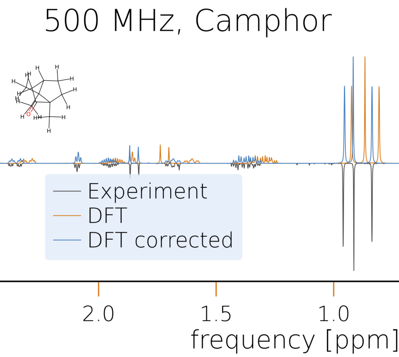
This data can be used to simulate the NMR spectra of all diastereomers as explained earlier and compare them to experimental ones, e.g., to that of neomenthol available here. Due to the limited accuracy of DFT calculations, it is not always straightforward to identify the correct isomer if the exact structure of the experimental measurement is unknown, but the comparison with all four possibilities will provide valuable insights for structure elucidation. Furthermore, the postprocessing module of HQS Spectrum Tools allows the user to modify the simulated spectrum to better match an experimental reference which will help to reduce the number of reasonable candidate structures.

Statistical evaluations

If, for the same set of molecular structures, two datasets with probe (e.g., calculations) and reference (e.g., experiments) NMR parameter data are available, the probe data can be evaluated quickly using the evaluate_shifts and evaluate_couplings functions to obtain the errors with respect to the reference data and resulting statistical measures. The functions take two MolecularDataSet objects, the first one being the probe dataset to be evaluated and the second one being the reference dataset to be evaluated against. The following basic example shows how to evaluate the calculated chemical shifts from CHESHIRE against the experimental data.

from hqs_nmr_parameters import evaluate_shifts
from hqs_nmr_parameters.cheshire import calculated, experimental_shifts_only

evaluation = evaluate_shifts(calculated, experimental_shifts_only)

The returned object (here evaluation) is an instance of type BenchmarkEvaluation and contains an attribute errors with a list of errors between the values from the probe and the reference dataset along with various properties providing statistical measures. For convenience, all relevant data from the evaluation can be printed with the print_all function.

evaluation.print_all()

The evaluate_couplings function can be used analogously for evaluating J-coupling constants. By default, all data points from both datasets are considered in the evaluation. However, for instance, if chemical shift values are available for more than one isotope, it makes sense to perform the evaluation only for data of a specific isotope. Therefore, the following isotope selection arguments are available:

• evaluate_shifts
  • isotope: Only data for this specified isotope (string or Isotope object) is considered in the evaluation.
• evaluate_couplings
  • isotopes: Only data for couplings between atoms of these specified isotopes (list of strings/Isotopes) is considered in the evaluation.
  • isotope_pairs: Only data for couplings between these specified isotope pairs (list of tuples of strings/Isotopes) is considered in the evaluation.
  • Both arguments can be combined, for example, the call

    evaluate_couplings(probe_dataset, ref_dataset, isotopes=["1H", "19F"], isotope_pairs=[("1H", "31P")])
    

    performs a J-coupling constant evaluation of the data in probe_dataset against that in ref_dataset for all of the following isotope pairs: ¹H–¹H, ¹H–¹⁹F, ¹⁹F–¹⁹F, and ¹H–³¹P.

These statistical evaluations can also directly be performed on a MolecularDataTable object. In this case, the functions evaluate_table_shifts and evaluate_table_couplings can be used by specifying the table and the label of the column that shall be used as reference dataset. They return a dictionary with the column labels of all other columns as keys and the corresponding BenchmarkEvaluation objects as values. The isotope selection options are the same as those shown above. An example for evaluating the calcualted and predicted chemical shifts in the CHESHIRE benchmark submodule is shown in the following:

from hqs_nmr_parameters import evaluate_table_shifts
from hqs_nmr_parameters.cheshire.benchmark import benchmark_1h

# The column labels are: "experimental shifts", "DFT", and "empirical prediction".
print("Column labels:", benchmark_1h.column_labels)
evaluations = evaluate_table_shifts(benchmark_1h, "experimental shifts", isotope="1H")

print("\nStatistics for calculated 1H NMR shifts:")
evaluations["DFT"].print_all()
print("\nStatistics for empirically predicted 1H NMR shifts:")
evaluations["empirical prediction"].print_all()

Input of molecular NMR parameters via a YAML file

NMR parameters for molecules can be provided in a YAML file. A brief summary of relevant YAML features is provided before proceeding to more detailed explanations and examples.

• Dictionaries in YAML are defined as key: value pairs. Most commonly, a dictionary contains one key/value pair per line:

  key 1: value 1
  key 2: value 2
  

• value 1 is interpreted as a string, 1 is interpreted as an integer and 1.0 is interpreted as a floating-point number. To avoid problems with special characters (e.g., square brackets), strings may be enclosed in single or double quotes (they have different meanings, and single quotes should be preferred for a literal interpretation of the string).
• Lists can be defined over multiple lines as:

  - item 1
  - item 2
  

  Lists can also be enclosed in square brackets: [item 1, item 2, item 3]. The nested list [[1, 2, 3], [4, 5, 6]] is equivalent to:

  - [1, 2, 3]
  - [4, 5, 6]
  

• Indentation is part of the syntax: key/value pairs or list entries over multiple lines need to have the same number of leading spaces (no tabs).
• Comments start with a hash, #.

Definition of the molecular structure

Definition using SMILES

A molecular structure needs to be provided along with its NMR parameters in order to get a complete molecular data input. The YAML input accepts one 2D structural representation, i.e., a SMILES string or a Molfile.

The simplest way to define a structure in the input file is through its SMILES representation. This is done using the key smiles, followed by a representation of the molecule. For acetic acid:

# Acetic acid defined using SMILES.
smiles: CC(=O)O

SMILES strings often contain square brackets [...]. In such cases, the string should be enclosed within quotes, '...', to avoid problems with the YAML parser.

Definition using a Molfile

Manual definition of increasingly large molecules using SMILES can be cumbersome. For example, the string representation of penicillin V would be:

smiles: 'CC1(C)S[C@@H]2[C@H](NC(=O)COc3ccccc3)C(=O)N2[C@H]1C(=O)O'

Instead, it is easier to draw a graphical representation such as the one below using one of many available proprietary or open-source packages.

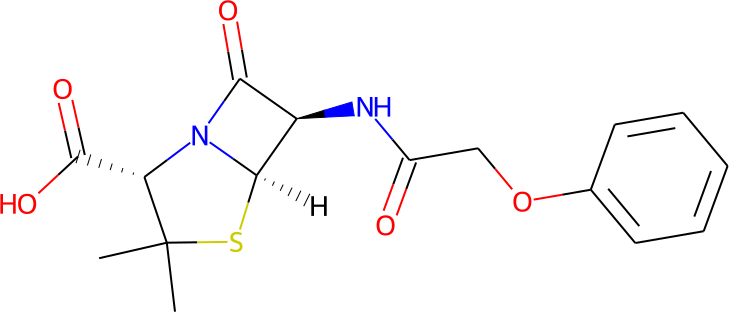
Such structural 2D representations are commonly stored in Molfiles. A molecule can be read from a Molfile by specifying the file name after the key molfile:

molfile: penicillin_v.mol

Note that the YAML input needs to contain either a Molfile or SMILES, but it is not possible to specify both at the same time. Both the V2000 and V3000 variants of the Molfile specification are supported in the input.

Hydrogens in the molecular structure

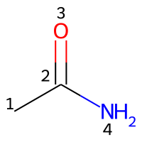
2D representations of molecular structures, whether as skeletal formulas or as SMILES, tend to omit hydrogens. Instead, the number of hydrogen atoms is inferred from the atomic valencies, especially those of the carbons. Any of the following three structures can be provided as a Molfile for the acrylamide molecule:

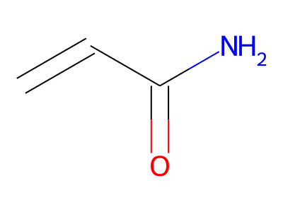
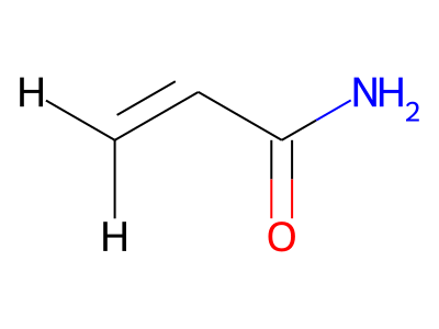
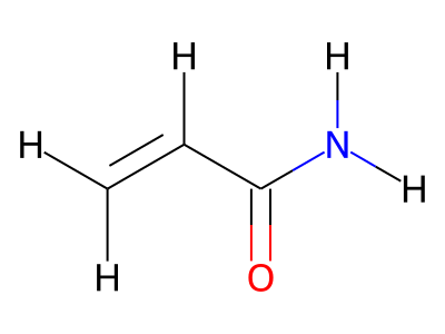
Where hydrogens are suppressed (not drawn out as separate atoms with a bond), their NMR parameters are specified through assignment to the respective skeletal atom. In the leftmost of the three structures shown above, it would not be possible to assign different parameters to the two protons in the CH₂ group. Instead, one of the two other structures shown above could be used to specify different parameters for those protons.

The only restriction with regard to hydrogens is that any skeletal atom can be connected either to suppressed or to stand-alone hydrogens, but not to a mixture of both. Thus, the following two structures would be rejected during input parsing:

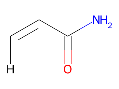
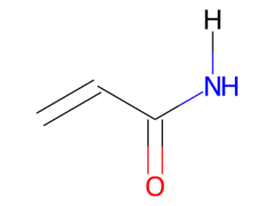
The structure to the left mixes a non-suppressed hydrogen with a suppressed "implicit" hydrogen (CH) on the carbon atom; the structure to the right mixes a non-suppressed hydrogen with a suppressed "explicit" hydrogen (NH) on the nitrogen atom.

Numbering of atoms

Atoms in the structural representation of the molecule are labelled with integers for the assignment of parameters. Indices can be counted starting from zero or from one. To avoid errors or misunderstandings, it is mandatory to specify a count from key in the input file, followed by either 0 or 1. The choice between those two options is entirely arbitrary.

An example for acetamide with atom counting starting from zero:

# Atom indices are 0, 1, 2, 3 in their order of appearance in the SMILES string.
smiles: CC(=O)N
count from: 0

An example for atom counting starting from one:

# Atom indices are 1, 2, 3, 4 in their order of appearance in the SMILES string.
smiles: CC(=O)N
count from: 1

The atoms in a molecule are indexed by their order of appearance in the Molfile. Acetamide may be represented by a Molfile with the following content (note that the file header must contain three lines):

     RDKit          2D

  4  3  0  0  0  0  0  0  0  0999 V2000
    0.0000    0.0000    0.0000 C   0  0  0  0  0  0  0  0  0  0  0  0
    1.2990    0.7500    0.0000 C   0  0  0  0  0  0  0  0  0  0  0  0
    1.2990    2.2500    0.0000 O   0  0  0  0  0  0  0  0  0  0  0  0
    2.5981   -0.0000    0.0000 N   0  0  0  0  0  0  0  0  0  0  0  0
  1  2  1  0
  2  3  2  0
  2  4  1  0
M  END

Counting the atoms starting from 1 (count from: 1), the appropriate indices are represented in the image below.

Chemical shifts

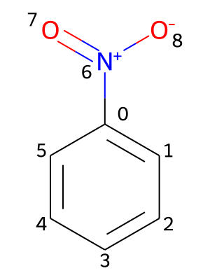
Providing chemical shifts will be illustrated using the nitrobenzene molecule as an example. Its molecular structure is contained in the file PhNO2.mol and shown in the picture below, including a numbering of its atoms.

All chemical shifts are specified under the key shifts. Additionally, the values need to be nested under keys representing isotopes, which contain the atomic mass number and the element symbol (e.g., 1H or 13C). For each isotope, the chemical shifts are provided in pairs of an atomic index and the associated value in ppm (parts per million):

# Structure with suppressed protons.
molfile: PhNO2.mol
count from: 0
shifts:
  # chemical shifts for protons in ppm
  1H:
    1: 8.23
    2: 7.56
    3: 7.71
    4: 7.56
    5: 8.23
  # chemical shifts for carbon-13 nuclei in ppm
  13C:
    0: 148.5
    1: 123.7
    2: 129.4
    3: 134.3
    4: 129.4
    5: 123.7

To assign chemical shifts for suppressed protons (that are not provided explicitly in the skeletal structure), the indices of the respective non-hydrogen atoms are used instead. All suppressed protons connected to the same atom are assigned an identical shift value.

If a Molfile contains hydrogens as standalone atoms, the chemical shifts are assigned to those protons using their respective atom indices. This is illustrated using the file PhNO2_allH.mol. Its structure is shown below.

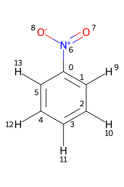
In this example, the ¹H shifts need to be assigned to atoms 9–13. Assigning them to atoms 1–5, as in the previous example, would produce an error.

# Structure with explicit protons.
molfile: PhNO2_allH.mol
count from: 0
shifts:
  # chemical shifts for protons in ppm
  1H:
    9: 8.23
    10: 7.56
    11: 7.71
    12: 7.56
    13: 8.23
  # chemical shifts for carbon-13 nuclei in ppm
  13C:
    0: 148.5
    1: 123.7
    2: 129.4
    3: 134.3
    4: 129.4
    5: 123.7

Indirect spin-spin coupling constants

Indirect spin-spin coupling constants are provided under the key J-couplings in the YAML file. Additionally, the coupling constant values need to be grouped together by isotopes. Keys for each combination of isotopes are combined as isotope1-isotope2: e.g., 1H-1H for coupling constants between two protons or 1H-13C for the associated heteronuclear coupling.

J-coupling constants in units of Hz for each combination of nuclei are provided as a list of lists with the following structure:

J-couplings:
  isotope1-isotope2:
    - [atom index 1, atom index 2, coupling constant in Hz]
    - [atom index 1, atom index 2, coupling constant in Hz]
    - [...]
  isotope1-isotope2:
    - [atom index 1, atom index 2, coupling constant in Hz]
    - [...]

The first atom index refers to the first isotope and the second atom index refers to the second isotope. As with shifts, values for suppressed hydrogens are assigned via the associated skeletal carbon or heteroatom. If multiple protons are connected to the same skeletal atom, they are assigned the same coupling constant. Inequivalent protons attached to the same skeletal atom, need to be specified explicitly as standalone atoms in the molecule definition, so that they can be referred to via their respective atom indices.

Examples

¹H parameters for propane with SMILES input

smiles: CCC
count from: 0
shifts:
  1H:
    0: 0.9
    1: 1.3
    2: 0.9
J-couplings:
  1H-1H:
    - [0, 1, 7.26]
    - [1, 2, 7.26]

The protons at the terminal CH₃ groups are assigned chemical shifts of 0.9 ppm each, and the protons of the central CH₂ group are given a value of 1.3 ppm. J-couplings between all protons of the neighboring CH₃ and CH₂ groups are assigned as 7.26 Hz. While an indirect spin-spin coupling interaction exists between equivalent protons within the CH₃ and CH₂ groups, it is not observed in the spectrum and the associated values are left out.

¹H parameters for acrylonitrile

The structure of acrylonitrile is provided as a Molfile in acrylonitrile.mol. Its depiction is shown below.

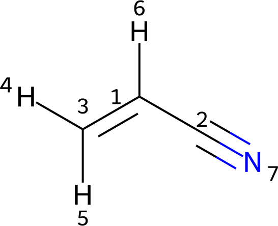
Since protons 4 and 5 are inequivalent, they are specified as standalone atoms with different parameters. In addition, hydrogen 6 is represented as a standalone atom, though suppressing it would also be an equally valid choice.

molfile: acrylonitrile.mol
count from: 1
shifts:
  1H:
    4: 5.79  # H(trans)
    5: 5.97  # H(cis)
    6: 5.48  # H(gem)
J-couplings:
  1H-1H:
    - [4, 5, 0.9]
    - [4, 6, 11.8]
    - [5, 6, 17.9]

Combined ¹H and ¹³C parameters for chloromethane

To illustrate the definition of heteronuclear coupling constants, the following example shows parameters for ¹³C-enriched chloromethane. The parameters include the shifts of the three protons and the ¹³C nucleus, as well as the coupling constants between these nuclei.

# CH3Cl with 13C, the hydrogens inside square brackets are implicit.
smiles: '[13CH3]Cl'
# C will have index 1 and Cl will have index 2
count from: 1
shifts:
  # Shifts of the three protons.
  1H:
    1: 3.05
  # Shift of carbon-13 in the molecule.
  13C:
    1: 25.6
J-couplings:
  # Coupling between the three protons (would normally not be observed).
  1H-1H:
    - [1, 1, -10.8]
  # Coupling between the three protons and the 13C atom.
  1H-13C:
    - [1, 1, 150.0]

Stored YAML files

For the molecules included in the examples module of the hqs-nmr-parameters package, YAML input files (and Molfiles when indicated as molecular structure) are available in the file system. To access them, use the following command, taking into account that each YAML file takes the name of its key in the dataset. The following shows the stored file and its data for acrylonitrile (with key "C2H3CN"):

from pathlib import Path
from hqs_nmr_parameters import examples

identifier = "C2H3CN"
acrylonitrile_yaml = Path(examples.__file__).parent.joinpath("parameters", identifier + ".yaml")
print(acrylonitrile_yaml.read_text())

name: Acrylonitrile
molfile: C2H3CN.mol
count from: 1
shifts:
  1H:
    4: 5.79  # H(trans)
    5: 5.97  # H(cis)
    6: 5.48  # H(gem)
J-couplings:
  1H-1H:
    - [4, 5, 0.9]
    - [4, 6, 11.8]
    - [5, 6, 17.9]
description: |
  1H parameters for acrylonitrile.
  Values were obtained from Hans Reich's Collection, NMR Spectroscopy.
  https://organicchemistrydata.org

As mentioned earlier, this data is already included as MolecularData instance:

from hqs_nmr_parameters.examples import molecules

identifier = "C2H3CN"
parameters = molecules[identifier]
print(parameters.shifts)
print(parameters.j_couplings)

[(3, 5.79), (4, 5.97), (5, 5.48)]
[((3, 4), 0.9), ((3, 5), 11.8), ((4, 5), 17.9)]

Therefore, even if the atom counting in the YAML file starts at 1, the numbering in MolecularData always starts at 0.

Reading and processing YAML input files

In HQS Spectrum Tools, a YAML file containing NMR parameters is parsed using the read_parameters_yaml function from the hqs-nmr-parameters package:

from hqs_nmr_parameters import read_parameters_yaml

parameters = read_parameters_yaml("input_file.yaml")

The read_parameters_yaml function can read the following keywords from a YAML file:

• name: An optional name of the molecule.
• shifts: Chemical shifts in format {isotope: {index: value}}.
• j_couplings/J-couplings: J-coupling values in format {isotope1-isotope2: [[index1, index2, value], ...]}.
• count from/count_from: Specifies whether to count atomic indices starting from zero or from one.
• smiles: SMILES string of the molecule (better enclosed in quotation marks).
• molfile: Path to a Molfile with the molecular structure. As mentioned above, only one representation entry can be set, i.e., either smiles or molfile.
• molblock: Compressed Molfile content (not in clear text).
• temperature: Temperature in K.
• solvent: Name of the solvent.
• description: Additional further description.

parameters is then an instance of the Pydantic MolecularData class.

Program components

The following components will enable you to quickly and conveniently run NMR spectrum calculations using HQS Spectrum Tools:

• A convenience function for quick and easy spectrum calculations.
• Different data types to serialize the input and output of NMR calculations.

While these functionalities are typically all you need, you may also browse through the API-documentation to check out all available features. However, we recommend to first go through the example notebooks to get an idea of how the package is typically used.

NMR spectra calculations

calculate_spectrum

For most use cases the calculate_spectrum function should be sufficient to perform NMR spectra calculations. By default, it uses the clustering approach discussed in the solver chapter. This approach is exact for molecules smaller than the specified maximum cluster size (set by default to 12) and for larger systems still accurate and efficient.

For a quick introduction to this method you can just read on, however, for a proper walkthrough of all the customization options check out the example notebooks.

The calculate_spectrum function takes as input an object with the molecular data of the system of interest which can be of type MolecularData or NMRParameters. The latter is derived from the former using the spin_system method and only stores the isotopes, chemical shifts and J-coupling values. The second input argument of calculate_spectrum is of type NMRCalculationParameters and stores all parameters necessary to specify a NMR spectrum calculation. For more details on these objects check out the corresponding sections molecular data and data types.

As part of HQS Spectrum Tools the hqs-nmr-parameters package containing example molecules is provided. You can calculate the spectrum for one of the example molecules simply as follows:

from hqs_nmr.calculate import calculate_spectrum
from hqs_nmr.datatypes import NMRCalculationParameters
from hqs_nmr_parameters.examples import molecules

# Obtain example molecule of datatype NMRParameters.
molecule_parameters = molecules["C3H8"].spin_system()

# Define the calculation parameters. The only required field is the magnetic
# field strength in Tesla.
calculation_parameters = NMRCalculationParameters(field_T=11.7433)

# Calculate the individual spin contributions of the spectrum.
nmr_result = calculate_spectrum(
    molecule_parameters,
    calculation_parameters
)

nmr_result is now an object of datatype NMRResultSpectrum1D and stores the calculated spectrum as well as the input to the calculation. The spectrum can be plotted as follows:

from hqs_nmr.visualization import plot_spectrum
from matplotlib import pyplot as plt

plot_spectrum(nmr_result.spectrum)
plt.show()

Data types

Molecular NMR parameters, spectra and calculation results are stored in Python objects in HQS Spectrum Tools. These data structures are all Pydantic data classes and the data can be accessed as attributes of the class. See NMRResultSpectrum1D for an example. Here we will elaborate on the datatypes defined within hqs-nmr, while in section Molecular data those defined in hqs-nmr-parameters are discussed.

Note that for the full signature of each datatype you can check out the API-documentation. Here we will just point out the most important attributes of each class.

NMRResultSpectrum1D

The NMRResultSpectrum1D is used to store all of the input and output of a NMR spectrum calculation when using the calculate_spectrum routine. It comprises:

• The molecular data used for the calculation, which can include the full data in a MolecularData object or only the NMR parameters with data type NMRParameters (molecule_parameters).

• All the parameters handed to calculate_spectrum in form of a NMRCalculationParameters object (calculation_parameters).

• The calculated spectrum of data type NMRSpectrum1D (spectrum).

Assuming we have obtained an object called result_spectrum of data type NMRResultSpectrum1D the attributes can be accessed as follows:

molecule_parameters = result.molecule_parameters
calculation_parameters = result.calculation_parameters
spectrum = result.spectrum

In the following we will elaborate on the data type of each of these objects in more detail.

NMRResultGreensFunction1D

The NMRResultGreensFunction1D is the analog data type to NMRResultSpectrum1D when using calculate_greens_function instead of calculate_spectrum. The only difference is that instead of the attribute spectrum, it has the attribute greens_function, which stores a NMRGreensFunction1D data type. For information on the difference between a spectrum and a Green's function check out the Math section.

Assuming we have an object called result_greens_function of data type NMRResultGreensFunction1D the greens_function attribute can be accessed as follows:

greens_function = result_greens_function.greens_function

NMRCalculationParameters

The NMRCalculationParameters data type stores all possible customization options when performing spectra calculations with calculate_spectrum or calculate_greens_function.

The only parameter the user always has to specify is the magnetic field strength in Tesla, so the most simple and often already sufficient instantiation of this data type may look as follows:

from hqs_nmr.datatypes import NMRCalculationParameters

calculation_parameters = NMRCalculationParameters(field_T=11.7433)

Another important option the user can set is the reference_isotope, which is the Isotope specified as Isotope(mass, symbol) to define the frequency of the rotating frame. Furthermore, the object contains multiple attributes allowing to improve the resolution. For a detailed explanation of the available customization options check out the tutorial notebooks or take a look at the API-documentation.

NMRSolverSettings

The NMRSolverSettings data type stores customization options specific for the solver backend. It is stored as an attribute of a NMRCalculationParameters object and typically does not need to be altered.

It is however important to know that by default a spin-dependent clustering of the molecule into overlapping clusters is performed (for details check here). This is an extremely accurate approximation especially at high field, however in some cases this might not be wanted. In these cases you can set the attribute perform_clustering=False, such that the spectrum of the entire molecule is calculated at once and symmetries will be exploited where applicable, but no approximations are made. Note that this can lead to a significant increase in runtime, so typically it is more advisable to increase the size of the clusters instead. To do so the attribute max_cluster_size has to be specified:

from hqs_nmr.datatypes import NMRSolverSettings

solver_settings = NMRSolverSettings(max_cluster_size=16)

To see all customization options check the API-documentation.

NMRSpectrum1D

The NMRSpectrum1D data type holds an NMR spectrum comprising the frequencies in ppm (omegas_ppm), an array with the individual spin contributions to the spectrum (spin_contributions) and the full-width-half-maximum in ppm (fwhm_ppm).

Assuming we have performed a NMR spectrum calculation using calculate_spectrum and obtained as output an NMRResultSpectrum1D object we called result_spectrum, we can obtain an object of data type NMRSpectrum1D as an attribute of this object:

spectrum = result_spectrum.spectrum

The spin_contributions are a $N_{\mathrm{spin}}\times N_{\mathrm{omegas}}$ NumPy array, where each row holds the contribution of the corresponding spin, i.e.:

spectrum.spin_contributions[0,:]

holds the contribution of the first spin (index 0). The total spectrum that would be measured experimentally can be calculated using

import numpy as np
np.sum(spectrum.spin_contributions, axis=0)

NMRGreensFunction1D

The NMRGreensFunction1D data type basically has the same attributes as NMRSpectrum1D, however spin_contributions is a complex array, as it stores the full NMR Green's function and not just the spectral function. This data type is typically only used if one wants to perform post-processing steps that require also the real part of the Green's function.

Assuming we have performed a NMR Green's function calculation using calculate_greens_function and obtained as output an NMRResultGreensFunction1D object called result_greens_function, we can obtain an object of data type NMRGreensFunction1D as an attribute of this object:

greens_function = result_greens_function.greens_function

The total spectrum can then be obtained as follows:

import numpy as np
np.sum(- np.imag(greens_function.spin_contributions), axis=0)

Serialization (Saving and Loading)

The data types described above have a common interface for data serialization. There exists a function called to_json common to all classes that can take a class object and a file name (with or without the full path) to store the data as a JSON file. For example, if we have an object called spectrum of the data class NMRSpectrum1D and want to save it as spectrum_data.json:

from hqs_nmr.datatypes import to_json

to_json(spectrum, "spectrum_data.json")

There is also the inverse method from_json to load the data again. It needs as additional information the type of class the JSON file has stored, e.g.:

from hqs_nmr.datatypes import from_json, NMRSpectrum1D

spectrum = from_json(NMRSpectrum1D, "spectrum_data.json")