Use cases
The HQStage Modules are centered around solving quantum mechanical systems. HQStage provides access to a wide range of example systems and Hamiltonians. There is great interest in solving these systems and Hamiltonains on quantum computers.
HQStage examples and modules will be available for three use cases:
- Nuclear magnetic resonance (HQS Spectrum Tools)
- Electron spectroscopy (HQS Quantum Solver)
- Magnetic response
As of now we have published the nuclear magnetic resonance (NMR) and the Electron spectroscopy use case. Magnetic resonance use cases will be published later in 2025.
Nuclear magnetic resonance
Expert users in NMR spectroscopy should use our HQStage modules HQS Spectrum Tools.
To get a feeling for NMR spectroscopy try out our end-to-end
product HQSpectrum.
See here for an example on how to use HQS Spectrum Tools NMR Hamiltonians with Qiskit to simulate NMR on a quantum computer.
In the following we will naswer the question why NMR is a good use case for quantum computers. For this we use our ITBQ use case evaluation.
I. Identify industry problem. NMR is a routine, cornerstone analytical technique for chemistry and pharma, used to determine molecular structure and to quantify mixtures (qNMR). Spectra encode structure through chemical shifts and J‑couplings, which depend on molecular environment (solvent, temperature, pH, field strength) and can be complex, especially for 1H spectra and at lower magnetic fields (benchtop devices).
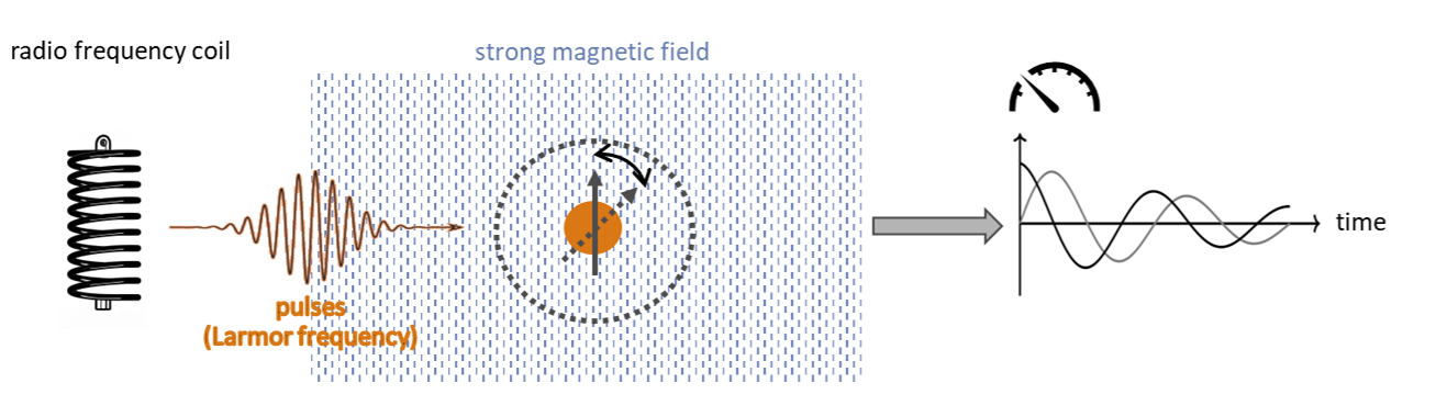
II. Transform to quantum. In the “transform to quantum” step we map molecules onto a quantum-mechanical spin model in which each nucleus is a spin-1/2 in a static magnetic field, and the spectrum is governed by Zeeman terms corrected by chemical shifts and by scalar J-couplings between spins; for diamagnetic molecules in liquids, direct dipolar couplings average out with molecular motion, while for macromolecules/solids they can matter. The resulting model is the Spin Hamiltonian:
Operationally, the transformation proceeds by generating 3D geometries and relevant conformers from molecular structure, optimizing them, computing shieldings and J-couplings (e.g., via DFT), Boltzmann-averaging parameters over the conformer ensemble, and converting shieldings to chemical shifts for use in the Hamiltonian; while these procedures are established and largely automated, integration into analysis workflows and accurate treatment of environmental effects still require manual checks. In HQS Spectrum Tools we provide a collection of pre-calculated spin models for a range of molecules with different size and chemical structures. Use these as a starting point for your NMR calculations - classical or on quantum computers. Rating: ★★★★☆.
III. Get the job done without the quantum computer.
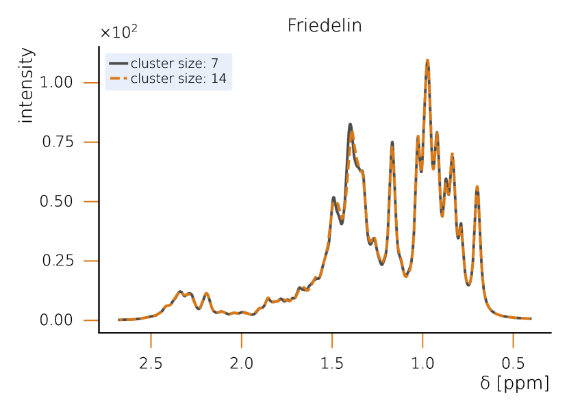
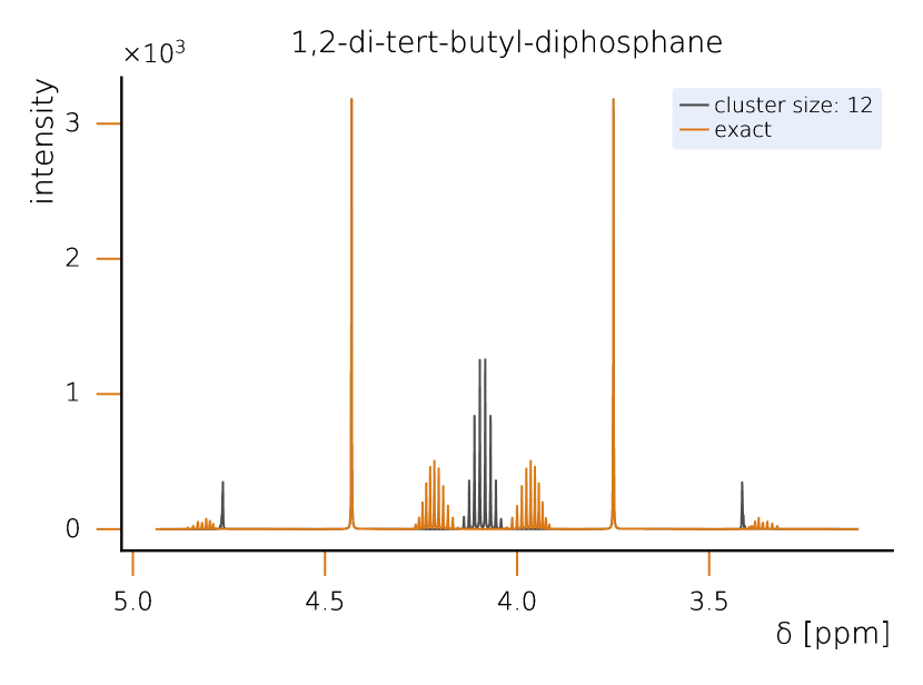
This section sets a clear classical baseline for quantum advantage in NMR simulations. Exact NMR dynamics scales exponentially with the number of spins, but with HQS Spectrum Tools practical, accurate results are routinely achieved by combining spin‑clustering (grouping strongly interacting spins) with symmetry reductions (e.g., local SU(2)), as implemented in the HQS Spectrum Tools and benchmarked against Spinach. Under typical high‑field conditions, these methods compute 1H spectra for organic molecules with tens of protons in minutes; for example, a 50‑spin Friedelin spectrum converges with clusters of about 8–12 spins. When correlations extend across the whole molecule, simple clustering can miss key features, yet symmetry‑aware exact modes still reproduce spectra for medium‑size systems, as shown for the 22‑spin 1,2‑di‑tert‑butyl‑diphosphane.
IV. NMR spectral prediction reduces to tracking the time‑dependent transverse magnetization of an N‑spin system, expressed as
While quantum computing offers an exponential advantage for NMR simulations, classical algorithms have also been developed to efficiently treat large spin systems. One particularly effective approach is spin clustering (see Fig. (2)), which reduces computational complexity by grouping strongly interacting spins together, enabling approximate solutions. In many cases, especially at high magnetic fields, this method can provide accurate results with cluster sizes of 8–12 spins, even for complex molecules. For example, in the case of Friedelin (Fig. 2), a 50-spin molecule, the cluster-based solver shows good convergence, with minimal spectral changes as the cluster size increases. This demonstrates that for certain systems with relatively weak spin correlations, spin clustering provides a feasible classical approach.
However, when strong correlations extend across the system, as in the case of 1,2-di-tert-butyl-diphosphane (Fig. 2), the limitations of spin clustering become apparent. This molecule consists of 22 coupled spins, where cluster approximations cannot fully capture the spin interactions. Instead, solving the system exactly requires the exploitation of local SU(2) symmetry, which significantly reduces the computational complexity while maintaining full accuracy. Without symmetry considerations, the problem would require the diagonalization of a -dimensional matrix, making classical exact diagonalization basically intractable. Given examples like 1,2-di-tert-butyl-diphosphane, it seams likely that parameters example and parameter regimes exist in which classical solutions remain challenging. At the same time it is clear that classical solvers can cover a large part of the relevant cases for NMR. Therefore we rate the probability to achieve quantum advantage with four stars (★★★★★).
Electron Spectroscopy (Singlet–Triplet Splitting)
Electron spectroscopy measures excited states of molecules. Depending on the setup, it can probe purely electronic excitations, vibrational structure on top of them, or their coupling. A particularly important quantity that these measurements access is the singlet–triplet energy splitting ΔEST between the lowest singlet (S1) and triplet (T1) states. In what follows we focus on accurately predicting ΔEST for realistic molecules.
I. Identify industry problem As an example for the importance of ΔEST we will discuss OLEDs. In commercial OLED displays and phones, the light‑emitting molecule (the emitter) is dissolved at low concentration in an organic‑semiconductor host. Its emission comes from the emitter’s lowest triplet state T1, so we must know where that level sits. The singlet–triplet splitting ΔEST fixes T1 once the singlet S1 is known, making accurate ΔEST a design‑critical number. For a stable, efficient device the emitter’s T1 must be lower than the triplet energies of the host and neighboring layers—i.e., not resonant with the host’s triplet manifold. If T1 is too close to, or above, the host triplet level, triplet excitons can hop from the emitter to the host via short‑range energy transfer or form interfacial charge‑transfer states. On the host these excitations are usually lost non‑radiatively, and they can also react with charge carriers or impurities to break chemical bonds. The outcomes are poorer efficiency, worse color purity and shorter lifetime. Hence, device engineers need reliable ΔEST predictions to place the emitter’s triplet safely below the host’s triplet energies. Similarly to OLEDs for displays we need ΔEST for other light emitting or absorbing materials.
II. Transform to quantum We start by building a sensible orbital basis for the molecule using Hartree–Fock (HF) or a very small CASSCF calculation to capture any obvious static correlation. From this basis we define an active space containing only the two frontier orbitals that control the singlet–triplet gap (two electrons in two orbitals). All remaining orbitals are “downfolded” with a random‑phase‑approximation (RPA) treatment: their collective response is represented as a set of effective harmonic resonators that screen and couple to the active space. This yields a compact effective Hamiltonian with a 4×4 electronic block (the two‑orbital problem) coupled to a handful of oscillators—i.e., a “two‑qubit plus oscillators” model. On a quantum computer the 4×4 block maps to two qubits and requires very shallow circuits; accuracy is dialed in by how many RPA modes we keep and by the truncation chosen for each mode. We then read out the singlet–triplet splitting ΔEST from this model (e.g., via energy estimation or shadow‑tomography style procedures), which will be discussed later in the quantum‑advantage section.
III. Get the job done without the quantum computer Our classical baseline is a straightforward multireference workflow built on PySCF with the Block DMRG solver. After preparing molecular geometries, we use the Active Space Finder (ASF) to choose the most important orbitals that control the singlet–triplet gap. The ASF is an open source tool developed by HQS in cooperation with Covestro and runs quick reference calculations, a DMRG calculation with low precision, and then proposes the smallest consistent set of “frontier” orbitals needed to form a consistent active space. This avoids trial‑and‑error and the need for manual expert guesses. With that active space fixed, we compute singlet and triplet energies using CASSCF; if more orbitals are needed for an accurate description, we swap the active‑space solver to DMRG via Block so we can treat larger spaces with the same overall setup. Finally, we include dynamical correlation on top of this multireference description using NEVPT2 or CASPT2. A major advantage as compared to our quantum computing approach is that CAS Methods are also routinely used to calculate various other energy difference of electronic states, which are also in principle accessible via electron spectroscopy. For more information about the ASF, read our paper.
IV. Show quantum advantage The RPA‑style reduction to a 4×4 electronic block coupled to a modest set of oscillators turns this into a problem whose quantum cost grows mainly with the number and truncation of those modes. So the problem is quite similar to the well known spin-boson problem, with a slightly enlarged spin system. Each boson can be in the cases we studied be mapped to a single qubit, since the RPA approximation depends on the occupation number of the bosons to stay low. But what is particularly interesting, is that the fact that we consider non-interacting boson, allows a large amount of mapping between the problem and the processor. It is well known in the study of spin boson systems, that the boson can be mapped to a 1-dimensional chain of bosons. This would allow simulation with constant depth even if the number of bosons increases ever further. Also many other mappings might be possible. Since we are looking at energy difference, it is also possible to extract the relevant quantities from time evolution under the system Hamiltonian. Here again we play towards the strength of quantum computing and can avoid e.g. variational approaches. A method like shadow spectroscpy should be sufficent to access all relevant results.